Chapter 2Delayed Public Signals and Asynchronous Learning

Public information often arrives after private learning has already occurred. Earnings releases, official statistics, and market-wide disclosures are public signals, but different agents may receive them with different delays after acting on partial private information. Delay creates a disclosure window during which a private action can move what others infer; at its known end the manipulation loses its effect.

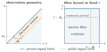
Extending the noise-state filtering and adjoint system to this timing requires centering the arriving delayed signal: at time $t$ , player $i$ observes $d Z_{t - Δ_{i}}$ with the part it could already predict subtracted, so the delayed signal arrives as an innovation. The resulting filter kernel has two births, the private-signal birth at $u = t$ and the public-signal birth at $u = t - Δ_{i}$ .

Linear-quadratic stochastic differential games with delay have been studied with the delay in the controls [28]; delayed observation of shared information is the delayed-sharing pattern of decentralized control [88, 111, 117]. Here the delay is in the observation of a public signal, so it enters the filtering and adjoint kernels rather than the state dynamics. The same equations cover the opposite timing, an action that is seen at once but takes effect after a lag $τ_{i}$ , as with time to build [70] or a purchase that is resold later. A delayed action changes the state dynamics and the first-order condition; the filter is untouched.

Section 2.1 sets up the delayed observation, Sections 2.2 and 2.3 derive the filter and verify it, and Section 2.4 prices the arrival in the adjoints and the first-order condition.

2.1Delayed observation structure

Fix a finite player set $I = {1, \dots, n}$ and choose an arbitrary player $i$ . Throughout this chapter, $i$ denotes the player whose filter or control is described, while $k \in I ∖ {i}$ denotes an opponent or another observer.

Player $i$ observes a private signal $d Y_{t}^{i} = (\overset{ˉ}{C}^{i, Y} (t) + \int_{0}^{t} C^{i, Y} (t, s) d W_{s}) d t + E^{i} d W_{t} . (2.1.1)$ There is also a public signal $d Z_{t} = (\overset{ˉ}{C}^{Z} (t) + \int_{0}^{t} C^{Z} (t, s) d W_{s}) d t + E^{Z} d W_{t} . (2.1.2)$ Each player may observe the public signal with a different delay. Player $i$ ’s delay is $Δ_{i} \geq 0$ , and $F_{t}^{i} = σ (Y_{r}^{i} : r \leq t) \lor σ (Z_{r} : r \leq t - Δ_{i}) .$ The common-delay case is $Δ_{1} = \dots = Δ_{n} = Δ$ . In applications the public drift kernel $C^{Z}$ may contain state, predictable-control, and uncontrolled components, $C^{Z} (t, s) = B_{X}^{Z} (t) X_{t} (s) + m \sum B_{m}^{Z} (t) D_{W, t}^{m} (s) + U_{t}^{Z} (s), (2.1.4)$ where control-dependent drifts use predictable controls $D_{t -}^{m}$ .

The state may also carry delayed control rows,

$d X_{t} = (B_{X}^{X} (t) X_{t} + m \sum B_{m}^{X} (t) D_{t}^{m} + m \sum \tilde{B}_{m}^{X} (t) D_{t - τ_{m}}^{m}) d t + σ (t) d W_{t}, D_{s}^{m} := 0 (s < 0), τ_{m} \geq 0, (2.1.5)$

with $\tilde{B}_{m}^{X} (s) := 0$ for $s > T$ . A control chosen at $t - τ_{m}$ depends only on noise born by then, so in the kernel state equation the delayed row is $\tilde{B}_{m}^{X} (t) 1_{{s \leq t - τ_{m}}} D_{W, t - τ_{m}}^{m} (s)$ , and the mean equation gains $\tilde{B}_{m}^{X} (t) \overset{ˉ}{D}_{t - τ_{m}}^{m}$ . The filtering results below do not change. $D_{t - τ_{m}}^{m}$ adds no martingale term to $d X$ ; the delayed rows therefore enter the drift kernels $C^{i, Y}$ and $C^{Z}$ only through $X_{t} (s)$ . With $\tilde{B}_{m}^{X} \equiv 0$ everything reduces to Chapter 1.

Assumption 2.1 (orthogonal delayed public news). The private and public martingale rows are normalized and orthogonal: $E^{i} E^{i, ⊤} = I, E^{Z} E^{Z, ⊤} = I, E^{i} E^{Z, ⊤} = 0. (2.1.6)$ Private rows do not directly measure $E^{Z} d W$ . Players may infer part of $E^{Z} d W_{t - Δ_{i}}$ indirectly through earlier drift effects, but this inference is predictable at $t -$ , so it changes only the drift of the arriving $Z$ -innovation, not its instantaneous covariance.

Let $s_{t}^{i} := t - Δ_{i}$ . At time $t$ , the arriving public increment for player $i$ is $d Z_{s_{t}^{i}}$ when $t \geq Δ_{i}$ . Define the pre-arrival projection of a primitive kernel $K$ by $(P_{t -}^{i} K) (u) := K (u) Π^{i} + 1_{{u < s_{t}^{i}}} K (u) Π^{Z} + \int_{0}^{t} K (r) F_{t -}^{i} (r, u) d r, (2.1.7)$ where $Π^{i} = E^{i, ⊤} E^{i}$ and $Π^{Z} = E^{Z, ⊤} E^{Z}$ . The strict inequality excludes the just-arriving coordinate $u = s_{t}^{i}$ . The complement $(I - P_{t -}^{i}) K$ is the part of $K$ that player $i$ has not resolved before the arrival.

The private unresolved row is $C_{t}^{i, Y} (u) := (I - P_{t -}^{i}) [C^{i, Y} (t, \cdot)] (u) . (2.1.8)$ Define the centered delayed-public innovation row $C_{t}^{i, Z} (u) := 1_{{t \geq Δ_{i}}} ((I - P_{t -}^{i}) [C^{Z} (s_{t}^{i}, \cdot)] (u) - E^{Z} F_{t -}^{i} (s_{t}^{i}, u)) . (2.1.9)$ Since $E^{Z} F_{t -}^{i} (t - Δ_{i}, \cdot)$ need not vanish, player $i$ also subtracts its predictable estimate of the arriving $Z$ -noise increment. The delayed-public innovation is $d I_{t}^{i, Z} := 1_{{t \geq Δ_{i}}} (d Z_{s_{t}^{i}} - E [d Z_{s_{t}^{i}} ∣ F_{t -}^{i}]) = 1_{{t \geq Δ_{i}}} E^{Z} d W_{s_{t}^{i}} + \int_{0}^{t} C_{t}^{i, Z} (u) d W_{u} d t . (2.1.10)$ Similarly, $d I_{t}^{i, Y} := d Y_{t}^{i} - E [d Y_{t}^{i} ∣ F_{t -}^{i}] = E^{i} d W_{t} + \int_{0}^{t} C_{t}^{i, Y} (u) d W_{u} d t . (2.1.11)$ By (2.1.6), $d I_{t}^{i, Y}$ and $d I_{t}^{i, Z}$ have block-identity instantaneous covariance and no mixed quadratic variation. Figure 2.1 shows the geometry.

Figure 2.1. Observation and filter geometry under delay. Left: a source coordinate enters the private innovation at $t = u$ and reaches player $i$ publicly at $t = u + Δ_{i}$ ; the strip between is the disclosure window. Right: the delayed public signal creates interior birth lines at $t - Δ_{i}$ .

2.2Filtering with delayed public signals

The theorem verifies a candidate kernel, taking the representation as given and deriving the equations it must satisfy. Existence of a kernel with the representation is part of the equilibrium fixed point and is not claimed here.

Theorem 2.2 (Filtering with a delayed public innovation row). For each $i \in I$ , let $Δ_{i}$ be a known constant delay, maintain Assumption 2.1, and suppose a deterministic kernel $F^{i}$ is such that the candidate noise-state has the representation $d_{u} W_{t}^{i} (u) = Π^{i} d W_{u} + 1_{{u < t - Δ_{i}}} Π^{Z} d W_{u} + (\int_{0}^{t} F_{t}^{i} (u, s) d W_{s}) d u . (2.2.1)$ Define $C^{i, Y}$ and $C^{i, Z}$ by (2.1.8) and (2.1.9). Away from the two birth lines $u = t$ and $u = t - Δ_{i}$ , $F^{i}$ satisfies $\partial_{t} F_{t}^{i} (u, s) = C_{t}^{i, Y} (u)^{⊤} C_{t}^{i, Y} (s) + C_{t}^{i, Z} (u)^{⊤} C_{t}^{i, Z} (s) . (2.2.2)$ The private signal creates the usual birth at $u = t$ , $F_{t}^{i} (u, t) = C_{t}^{i, Y} (u)^{⊤} E^{i}, F_{t}^{i} (t, u) = E^{i, ⊤} C_{t}^{i, Y} (u), (2.2.3)$ and the delayed public signal creates a second birth at $s_{t}^{i} = t - Δ_{i}$ , the coordinate whose public news arrives at $t$ , $F_{t}^{i} (u, s_{t}^{i})_{Z} = C_{t}^{i, Z} (u)^{⊤} E^{Z}, F_{t}^{i} (s_{t}^{i}, u)_{Z} = E^{Z, ⊤} C_{t}^{i, Z} (u) . (2.2.4)$ Equivalently, with noncausal rows and empty integrals equal to zero, $F_{t}^{i} (u, s) = C_{s}^{i, Y} (u)^{⊤} E^{i} + E^{i, ⊤} C_{u}^{i, Y} (s) + 1_{{s + Δ_{i} \leq t}} C_{s + Δ_{i}}^{i, Z} (u)^{⊤} E^{Z} + 1_{{u + Δ_{i} \leq t}} E^{Z, ⊤} C_{u + Δ_{i}}^{i, Z} (s) + \int_{m a x {u, s}}^{t} C_{r}^{i, Y} (u)^{⊤} C_{r}^{i, Y} (s) d r + \int_{m a x {u, s}}^{t} C_{r}^{i, Z} (u)^{⊤} C_{r}^{i, Z} (s) d r . (2.2.5)$ With $F^{i}$ given by (2.2.5), (2.2.1) is the conditional expectation $E [W_{u} ∣ F_{t}^{i}]$ .

2.3Filtering derivation

The argument follows the proof of the baseline filtering theorem, Theorem 1.5. The only new ingredient is that the test martingale has two orthogonal measurement rows and the delayed public news is the centered innovation (2.1.10).

Exponential tests

Fix deterministic test functions $r_{Y}, r_{Z}$ and define $d ϕ_{t} = i ϕ_{t} [(d I_{t}^{i, Y})^{⊤} r_{Y} (t) + (d I_{t}^{i, Z})^{⊤} r_{Z} (t)], ϕ_{0} = 1. (2.3.1)$ The candidate $W_{t}^{i} (u)$ is the conditional expectation of $W_{u}$ if and only if $E [W_{t}^{i} (u) ϕ_{t}] = E [W_{u} ϕ_{t}] for all r_{Y}, r_{Z} . (2.3.2)$

Left-hand side

Write the candidate innovation-form dynamics for a fixed coordinate $u$ as $d_{t} W_{t}^{i} (u) = B_{Y}^{W, i} (u, t) d I_{t}^{i, Y} + B_{Z}^{W, i} (u, t) d I_{t}^{i, Z} . (2.3.3)$ Since the two innovation rows have no mixed quadratic variation, Itô’s product rule gives $d (W_{t}^{i} (u) ϕ_{t}) = i W_{t}^{i} (u) ϕ_{t} (d I_{t}^{i, Y})^{⊤} r_{Y} (t) + i W_{t}^{i} (u) ϕ_{t} (d I_{t}^{i, Z})^{⊤} r_{Z} (t) + ϕ_{t} B_{Y}^{W, i} (u, t) d I_{t}^{i, Y} + ϕ_{t} B_{Z}^{W, i} (u, t) d I_{t}^{i, Z} + i ϕ_{t} B_{Y}^{W, i} (u, t) r_{Y} (t) d t + i ϕ_{t} B_{Z}^{W, i} (u, t) r_{Z} (t) d t .$ Using (2.1.11)–(2.1.10) to collect the $d t$ terms, $\frac{d}{d t} E [W_{t}^{i} (u) ϕ_{t}] = i E [ϕ_{t} (W_{t}^{i} (u) \int_{0}^{t} C_{t}^{i, Y} (r) d W_{r}^{⊤} + B_{Y}^{W, i} (u, t))] r_{Y} (t) + i E [ϕ_{t} (W_{t}^{i} (u) \int_{0}^{t} C_{t}^{i, Z} (r) d W_{r}^{⊤} + B_{Z}^{W, i} (u, t))] r_{Z} (t) . (2.3.5)$ No additional predictable residual appears because $I^{i, Y}$ and $I^{i, Z}$ are already centered relative to $F_{t -}^{i}$ .

Right-hand side

For the private row, $\frac{1}{d t} E [W_{u} (d I_{t}^{i, Y})^{⊤} ∣ F_{t -}^{i}] = = E [W_{u} \int_{0}^{t} C_{t}^{i, Y} (r) d W_{r}^{⊤} ∣ F_{t -}^{i}] + E^{i, ⊤} 1_{{u \geq t}} W_{t -}^{i} (u) \int_{0}^{t} C_{t}^{i, Y} (r) d W_{t -}^{i} (r)^{⊤} + \int_{0}^{t} \partial_{r} C_{t -}^{i} (u, r) C_{t}^{i, Y} (r)^{⊤} d r + E^{i, ⊤} 1_{{u \geq t}}, (2.3.6)$ where $C_{t}^{i} (u, r) = Cov (W_{u}, W_{r} ∣ F_{t}^{i})$ . For the delayed public signal, the same calculation applies to the centered innovation (2.1.10). The martingale part arrives at $s_{t}^{i}$ and the drift row is $C^{i, Z}$ , so $\frac{1}{d t} E [W_{u} (d I_{t}^{i, Z})^{⊤} ∣ F_{t -}^{i}] = W_{t -}^{i} (u) \int_{0}^{t} C_{t}^{i, Z} (r) d W_{t -}^{i} (r)^{⊤} + \int_{0}^{t} \partial_{r} C_{t -}^{i} (u, r) C_{t}^{i, Z} (r)^{⊤} d r + E^{Z, ⊤} 1_{{t \geq Δ_{i}}} 1_{{u \geq s_{t}^{i}}} . (2.3.7)$ Combining,

$\frac{d}{d t} E [W_{u} ϕ_{t}] = i E [ϕ_{t} (W_{t}^{i} (u) \int_{0}^{t} C_{t}^{i, Y} (r) d W_{t}^{i} (r)^{⊤} + \int_{0}^{t} \partial_{r} C_{t}^{i} (u, r) C_{t}^{i, Y} (r)^{⊤} d r + E^{i, ⊤} 1_{{u \geq t}})] r_{Y} (t) * + i E [ϕ_{t} (W_{t}^{i} (u) \int_{0}^{t} C_{t}^{i, Z} (r) d W_{t}^{i} (r)^{⊤} + \int_{0}^{t} \partial_{r} C_{t}^{i} (u, r) C_{t}^{i, Z} (r)^{⊤} d r + E^{Z, ⊤} 1_{{t \geq Δ_{i}}} 1_{{u \geq s_{t}^{i}}})] r_{Z} (t) . (2.3.8)$

Coefficient matching

Matching (2.3.5) and (2.3.8) for arbitrary $r_{Y}, r_{Z}$ gives $B_{Y}^{W, i} (u, t) B_{Z}^{W, i} (u, t) = \int_{0}^{t} \partial_{r} C_{t}^{i} (u, r) C_{t}^{i, Y} (r)^{⊤} d r + E^{i, ⊤} 1_{{u \geq t}}, = \int_{0}^{t} \partial_{r} C_{t}^{i} (u, r) C_{t}^{i, Z} (r)^{⊤} d r + E^{Z, ⊤} 1_{{t \geq Δ_{i}}} 1_{{u \geq s_{t}^{i}}} . (2.3.9) (2.3.10)$ Differentiating these expressions in the source time $u$ gives, away from jumps, $d_{t} (d_{u} W_{t}^{i} (u)) = C_{t}^{i, Y} (u)^{⊤} d I_{t}^{i, Y} d u + C_{t}^{i, Z} (u)^{⊤} d I_{t}^{i, Z} d u . (2.3.11)$ Equation (2.3.9) jumps at $u = t$ , giving the private-signal birth, and (2.3.10) jumps at $u = s_{t}^{i}$ , giving the public-signal birth.

Primitive-shock expansion and the two birth terms

Integrating (2.3.11) over observation times gives $d_{u} W_{t}^{i} (u) = E^{i, ⊤} d I_{u}^{i, Y} + 1_{{u + Δ_{i} \leq t}} E^{Z, ⊤} d I_{u + Δ_{i}}^{i, Z} + (\int_{u}^{t} C_{r}^{i, Y} (u)^{⊤} d I_{r}^{i, Y}) d u + (\int_{u}^{t} C_{r}^{i, Z} (u)^{⊤} d I_{r}^{i, Z}) d u . (2.3.12)$ Substitute (2.1.11) and (2.1.10). The direct private term is $E^{i, ⊤} d I_{u}^{i, Y} = Π^{i} d W_{u} + E^{i, ⊤} \int_{0}^{u} C_{u}^{i, Y} (s) d W_{s} d u .$ The direct delayed public term is $1_{{u + Δ_{i} \leq t}} E^{Z, ⊤} d I_{u + Δ_{i}}^{i, Z} = 1_{{u + Δ_{i} \leq t}} Π^{Z} d W_{u} + 1_{{u + Δ_{i} \leq t}} E^{Z, ⊤} \int_{0}^{u + Δ_{i}} C_{u + Δ_{i}}^{i, Z} (s) d W_{s} d u .$ The accumulated martingale updates contribute $\int_{u}^{t} C_{r}^{i, Y} (u)^{⊤} E^{i} d W_{r} d u, \int_{m a x {0, u - Δ_{i}}}^{t - Δ_{i}} C_{s + Δ_{i}}^{i, Z} (u)^{⊤} E^{Z} d W_{s} d u .$ The accumulated drift updates contribute, by stochastic Fubini, $\int_{0}^{t} (\int_{m a x {u, s}}^{t} C_{r}^{i, Y} (u)^{⊤} C_{r}^{i, Y} (s) d r) d W_{s} d u, \int_{0}^{t} (\int_{m a x {u, s}}^{t} C_{r}^{i, Z} (u)^{⊤} C_{r}^{i, Z} (s) d r) d W_{s} d u .$ Collecting the coefficient of $d W_{s} d u$ gives (2.2.5). The singular direct terms give the two direct pieces in (2.2.1). The candidate representation satisfies the test identities (2.3.2); uniqueness follows from Itô isometry as in the proof of Theorem 1.5.

2.4First variations and delayed-public adjoints

A deviation misleads private learners today, but the manipulated component resurfaces when the public news arrives at delay $Δ_{k}$ . Player $i$ pays for moving the drift of the delayed public signal when that signal reaches opponent $k$ , and the belief price $H^{k, i}$ jumps at that date; together these are the marginal cost of that second effect. Each opponent now carries two observation rows, the private row and the centered delayed-public innovation.

Fix the deviating player $i$ and freeze opponents’ strategy maps and filters. For $k \neq = i$ , write $δ w_{s}^{k} (u)$ for the density variation of opponent $k$ ’s noise-state and $δ X_{s}$ for the physical-state variation. The induced opponent-control variation is $δ D_{s}^{k} = \int_{0}^{s} D_{s}^{k} (u) δ w_{s}^{k} (u) d u . (2.4.1)$ Opponent $k$ observes at time $s$ the public signal generated at source time $q_{k} = s_{s}^{k} = s - Δ_{k}$ . Write $δ b_{q_{k}}^{Z}$ for the variation of the predictable drift of that public signal. In the affine example $b_{q_{k}}^{Z} = B_{X}^{Z} (q_{k}) X_{q_{k}} + \sum_{m} B_{m}^{Z} (q_{k}) D_{q_{k} -}^{m} + U_{q_{k}}^{Z}$ , this means $δ b_{q_{k}}^{Z} = B_{X}^{Z} (q_{k}) δ X_{q_{k}} + m \neq = i \sum B_{m}^{Z} (q_{k}) \int_{0}^{q_{k}} D_{q_{k}}^{m} (r) δ w_{q_{k}}^{m} (r) d r, (2.4.2)$ with the right-hand side zero if $q_{k}$ lies before the initial perturbation date. The deviating player’s own instantaneous effect through $B_{i}^{Z} (q_{k}) D_{q_{k}}^{i}$ stays out of the forward variation system and enters the first-order condition below directly.

Forward first-variation system

Opponent $k$ ’s private residual is $η_{s}^{k, Y} := B_{X}^{Y, k} (s) (δ X_{s} - \int_{0}^{s} X_{s} (r) δ w_{s}^{k} (r) d r) . (2.4.3)$ The subtraction leaves the part of the state variation opponent $k$ has not yet inferred. The centered delayed-public residual is $η_{s}^{k, Z} := 1_{{s \geq Δ_{k}}} (δ b_{q_{k}}^{Z} - \int_{0}^{s} C^{Z} (q_{k}, r) δ w_{s -}^{k} (r) d r - E^{Z} δ w_{s -}^{k} (q_{k})), q_{k} = s - Δ_{k} . (2.4.4)$ The last term is the first-variation counterpart of the centering correction $- E^{Z} F_{s -}^{k} (q_{k}, \cdot)$ in the delayed-public innovation.

Existing noise-state coordinates satisfy $\partial_{s} δ w_{s}^{k} (u) = C_{s}^{k, Y} (u)^{⊤} η_{s}^{k, Y} + C_{s}^{k, Z} (u)^{⊤} η_{s}^{k, Z}, u < s, (2.4.5)$ with two birth conditions, one at the current date and one at the arrival date, $δ w_{s}^{k} (s)_{Y} = E^{k, ⊤} η_{s}^{k, Y}, δ w_{s}^{k} (s - Δ_{k})_{Z} = 1_{{s \geq Δ_{k}}} E^{Z, ⊤} η_{s}^{k, Z} . (2.4.6)$ The physical variation satisfies

$\frac{d}{d s} δ X_{s} = B_{X}^{X} (s) δ X_{s} + k \neq = i \sum B_{k}^{X} (s) \int_{0}^{s} D_{s}^{k} (u) δ w_{s}^{k} (u) d u + k \neq = i \sum \tilde{B}_{k}^{X} (s) \int_{0}^{s - τ_{k}} D_{s - τ_{k}}^{k} (u) δ w_{s - τ_{k}}^{k} (u) d u, (2.4.7)$

where $δ w_{r}^{k} \equiv 0$ before the perturbation date. The last sum in (2.4.7) is what opponent $k$ decided $τ_{k}$ ago, on the beliefs it held then. The deviating player’s spike now produces two impulses, $δ X_{t} = v := B_{i}^{X} (t) z$ when it acts and a jump $\tilde{v} := \tilde{B}_{i}^{X} (t + τ_{i}) z$ at the effect date. Equations (2.4.3)–(2.4.7) are the delayed-public analogue of the baseline forward variation system.

Forward transfer functions

For $s \geq t$ , define the forward transfer functions by the response to initial data $(δ X_{t}, δ w_{t}^{m} (\cdot))$ , $m \neq = i$ : $δ X_{s} δ w_{s}^{k} (r) = Φ^{XX} (s, t) v + m \neq = i \sum \int_{0}^{t} Φ^{X m} (s, t, u) δ w_{t}^{m} (u) d u, = Φ^{k X} (s, t, r) v + m \neq = i \sum \int_{0}^{t} Φ^{km} (s, t, r, u) δ w_{t}^{m} (u) d u . (2.4.8) (2.4.9)$ The initial conditions are $Φ^{XX} (t, t) = I, Φ^{k X} (t, t, r) = 0, Φ^{X m} (t, t, u) = 0, Φ^{km} (t, t, r, u) = 1_{{k = m}} δ (r - u), (2.4.10)$ where the last identity holds weakly.

Define the residual transfer coefficients obtained by substituting (2.4.8)–(2.4.9) into (2.4.3)–(2.4.4). For a physical initial perturbation $v$ , set $Y^{k X} (s, t) := B_{X}^{Y, k} (s) (Φ^{XX} (s, t) - \int_{0}^{s} X_{s} (r) Φ^{k X} (s, t, r) d r), (2.4.11)$ and $Z^{k X} (s, t) := 1_{{s \geq Δ_{k}}} [δ b_{q_{k}; t}^{Z, X} - \int_{0}^{s} C^{Z} (q_{k}, r) Φ^{k X} (s -, t, r) d r - E^{Z} Φ^{k X} (s -, t, q_{k})], q_{k} = s - Δ_{k}, (2.4.12)$ where $δ b_{q_{k}; t}^{Z, X} := B_{X}^{Z} (q_{k}) Φ^{XX} (q_{k}, t) + ℓ \neq = i \sum B_{ℓ}^{Z} (q_{k}) \int_{0}^{q_{k}} D_{q_{k}}^{ℓ} (r) Φ^{ℓ X} (q_{k}, t, r) d r, (2.4.13)$ with all transfer functions at $q_{k} < t$ read as zero in the first two terms. Similarly, for an initial belief perturbation in block $m$ , $Y^{km} (s, t, u) := B_{X}^{Y, k} (s) (Φ^{X m} (s, t, u) - \int_{0}^{s} X_{s} (r) Φ^{km} (s, t, r, u) d r), (2.4.14)$ and $Z^{km} (s, t, u) := 1_{{s \geq Δ_{k}}} [δ b_{q_{k}; t}^{Z, km} (u) - \int_{0}^{s} C^{Z} (q_{k}, r) Φ^{km} (s -, t, r, u) d r - E^{Z} Φ^{km} (s -, t, q_{k}, u)], (2.4.15)$ where $δ b_{q_{k}; t}^{Z, km} (u) := B_{X}^{Z} (q_{k}) Φ^{X m} (q_{k}, t, u) + ℓ \neq = i \sum B_{ℓ}^{Z} (q_{k}) \int_{0}^{q_{k}} D_{q_{k}}^{ℓ} (r) Φ^{ℓ m} (q_{k}, t, r, u) d r . (2.4.16)$

The transfer functions solve the forward equations $\partial_{s} Φ^{XX} (s, t) \partial_{s} Φ^{X m} (s, t, u) \partial_{s} Φ^{k X} (s, t, r) \partial_{s} Φ^{km} (s, t, r, u) = B_{X}^{X} (s) Φ^{XX} (s, t) + k \neq = i \sum B_{k}^{X} (s) \int_{0}^{s} D_{s}^{k} (r) Φ^{k X} (s, t, r) d r + k \neq = i \sum \tilde{B}_{k}^{X} (s) \int_{0}^{s - τ_{k}} D_{s - τ_{k}}^{k} (r) Φ^{k X} (s - τ_{k}, t, r) d r, = B_{X}^{X} (s) Φ^{X m} (s, t, u) + k \neq = i \sum B_{k}^{X} (s) \int_{0}^{s} D_{s}^{k} (r) Φ^{km} (s, t, r, u) d r + k \neq = i \sum \tilde{B}_{k}^{X} (s) \int_{0}^{s - τ_{k}} D_{s - τ_{k}}^{k} (r) Φ^{km} (s - τ_{k}, t, r, u) d r, = C_{s}^{k, Y} (r)^{⊤} Y^{k X} (s, t) + C_{s}^{k, Z} (r)^{⊤} Z^{k X} (s, t), = C_{s}^{k, Y} (r)^{⊤} Y^{km} (s, t, u) + C_{s}^{k, Z} (r)^{⊤} Z^{km} (s, t, u), (2.4.17) (2.4.18) (2.4.19) (2.4.20)$ for old-history coordinates, those already born and away from the two birth lines, together with the two boundary updates $Φ^{k X} (s, t, s)_{Y} Φ^{km} (s, t, s, u)_{Y} Φ^{k X} (s, t, s - Δ_{k})_{Z} Φ^{km} (s, t, s - Δ_{k}, u)_{Z} = E^{k, ⊤} Y^{k X} (s, t), = E^{k, ⊤} Y^{km} (s, t, u), = 1_{{s \geq Δ_{k}}} E^{Z, ⊤} Z^{k X} (s, t), = 1_{{s \geq Δ_{k}}} E^{Z, ⊤} Z^{km} (s, t, u) . (2.4.21) (2.4.22)$ Transfer functions with a time argument below $t$ are zero, so the delayed rows are inactive until $s = t + τ_{k}$ . The deviating player’s delayed impulse stays outside the forward variation system; by linearity it contributes $Φ^{XX} (s, t + τ_{i}) \tilde{v}$ .

2.4.1State price, belief prices, and cost variation

Let $L_{s}^{i} := G^{XX, i} (s) X_{s} + G_{s}^{X, i} + G^{X D, i} (s) D_{s}^{i}, L_{T}^{i} := G^{XX, i} (T) X_{T} + G_{T}^{X, i} .$ $L_{s}^{i}$ and $L_{T}^{i}$ are the running and terminal marginal costs of the physical state. Pairing the forward state response with future marginal costs gives the state price and the belief prices: $H_{t}^{X, i} H_{t}^{k, i} (u) := \int_{t}^{T} Φ^{XX} (s, t)^{⊤} L_{s}^{i} d s + Φ^{XX} (T, t)^{⊤} L_{T}^{i}, := \int_{t}^{T} Φ^{X k} (s, t, u)^{⊤} L_{s}^{i} d s + Φ^{X k} (T, t, u)^{⊤} L_{T}^{i}, k \neq = i . (2.4.24) (2.4.25)$ Here $Φ^{X k}$ is the state response to an initial perturbation of opponent $k$ ’s noise-state coordinate.

For a control spike $z \in L^{2} (Ω, F_{t}^{i}; R^{d})$ , the normalized first variation of player $i$ ’s cost is

$δ J_{t}^{i} (z) = E [z^{⊤} (G^{DD, i} (t) D_{t}^{i} + G^{D X, i} (t) X_{t} + B_{i}^{X} (t)^{⊤} H_{t}^{X, i} + 1_{{t + τ_{i} \leq T}} \tilde{B}_{i}^{X} (t + τ_{i})^{⊤} H_{t + τ_{i}}^{X, i}) ∣ F_{t}^{i}] + E z^{⊤} B_{i}^{Z} (t)^{⊤} k \neq = i \sum 1_{{t + Δ_{k} \leq T}} (B^{k, Z} H^{k, i})_{t + Δ_{k} \leftarrow t} ∣ F_{t}^{i} (2.4.26)$

when the deviating player’s predictable action enters the public-signal drift through $B_{i}^{Z} (t) D_{t -}^{i}$ . If $B_{i}^{Z} \equiv 0$ , the second line drops out. The new term in the first line is the state price at the effect date.

Backward equations

The two birth conditions of the forward system, at the current date and at the arrival date, enter the backward system through two forms of the filter contraction $B$ of Chapter 1, equation (1.4.9), which contracts a belief price against the observer’s own filter. The filter contraction of the belief price is $B^{k} H_{t}^{k, i} = E^{k} H_{t}^{k, i} (t) + \int_{0}^{t} C_{t}^{k, Y} (r) H_{t}^{k, i} (r) d r . (2.4.27)$ This is the price, for player $i$ , of moving opponent $k$ ’s private signal-source drift at time $t$ . For the public row generated at source time $s$ and observed by opponent $k$ at $s + Δ_{k}$ , the delayed contraction $B^{k, Z}$ is built from the centered public innovation $(E^{Z}, C^{k, Z})$ ; player $i$ pays it at the arrival date $s + Δ_{k}$ , projected on information at the source time $s$ : $(B^{k, Z} H^{k, i})_{s + Δ_{k} \leftarrow s} := 1_{{s + Δ_{k} \leq T}} (E^{Z} H_{s + Δ_{k}}^{k, i} (s) + \int_{0}^{s + Δ_{k}} C_{s + Δ_{k}}^{k, Z} (r) H_{s + Δ_{k}}^{k, i} (r) d r) . (2.4.28)$ This is the price of moving the drift of the delayed public signal row generated at source time $s$ , paid when the row reaches opponent $k$ . The first term in each display is the transpose of the birth condition (2.4.6); the integral term is the transpose of the drift update (2.4.5).

Differentiating the transfer representations (2.4.24)–(2.4.25), using the forward equations (2.4.17)–(2.4.22), and collecting the coefficients of $δ X$ and $δ w^{k}$ gives the equations below. With delayed rows the forward system is a linear delay system, whose adjoint carries advanced arguments; the coefficient of $δ w_{t}^{k} (u)$ then collects the state price at $t$ and at $t + τ_{k}$ . $\frac{d}{d t} H_{t}^{X, i} = - L_{t}^{i} - B_{X}^{X} (t)^{⊤} H_{t}^{X, i} - k \neq = i \sum V_{t}^{k, i}, (2.4.29)$ where $V_{t}^{k, i} = B_{X}^{Y, k} (t)^{⊤} B^{k} H_{t}^{k, i} + 1_{{t + Δ_{k} \leq T}} B_{X}^{Z} (t)^{⊤} (B^{k, Z} H^{k, i})_{t + Δ_{k} \leftarrow t} . (2.4.30)$ The belief price satisfies, for old-history coordinates other than the one whose public news arrives at $t$ , $\frac{d}{d t} H_{t}^{k, i} (u) = - (B_{k}^{X} (t) D_{t}^{k} (u))^{⊤} H_{t}^{X, i} - 1_{{t + τ_{k} \leq T}} (\tilde{B}_{k}^{X} (t + τ_{k}) D_{t}^{k} (u))^{⊤} H_{t + τ_{k}}^{X, i} + X_{t} (u)^{⊤} B_{X}^{Y, k} (t)^{⊤} B^{k} H_{t}^{k, i} + 1_{{t \geq Δ_{k}}} C^{Z} (t - Δ_{k}, u)^{⊤} (B^{k, Z} H^{k, i})_{t \leftarrow t - Δ_{k}} - k^{'} \neq = i \sum 1_{{t + Δ_{k^{'}} \leq T}} (B_{k}^{Z} (t) D_{t}^{k} (u))^{⊤} (B^{k^{'}, Z} H^{k^{'}, i})_{t + Δ_{k^{'}} \leftarrow t} . (2.4.31)$ When the news about the coordinate $u = t$ arrives, at time $t + Δ_{k}$ , the centered delayed-public innovation adds a jump, dual to the centering term $- E^{Z} δ w_{s -}^{k} (q_{k})$ in (2.4.4): $H_{t + Δ_{k} -}^{k, i} (t) = H_{t + Δ_{k} +}^{k, i} (t) - E^{Z, ⊤} (B^{k, Z} H^{k, i})_{t + Δ_{k} \leftarrow t} . (2.4.32)$ Equations (2.4.29)–(2.4.32) reduce to the baseline adjoint system when the delayed public signal is absent and $\tilde{B}^{X} \equiv 0$ . The second term in (2.4.31) is the delayed-action term, the state price at $t + τ_{k}$ , which a backward sweep has already formed. Equation (2.4.29) is unchanged because a delayed control is noise-state linear, so its variation in (2.4.7) is driven by $δ w_{s - τ_{m}}^{m}$ and not by $δ X_{s}$ .

First-order condition

Since the best-response problem is strictly convex in the deviating player’s $L^{2}$ control, stationarity of (2.4.26) for every $z \in L^{2} (Ω, F_{t}^{i}; R^{d})$ gives $G^{DD, i} (t) D_{t}^{i} + E [G^{D X, i} (t) X_{t} + B_{i}^{X} (t)^{⊤} H_{t}^{X, i} + 1_{{t + τ_{i} \leq T}} \tilde{B}_{i}^{X} (t + τ_{i})^{⊤} H_{t + τ_{i}}^{X, i} + B_{i}^{Z} (t)^{⊤} k \neq = i \sum 1_{{t + Δ_{k} \leq T}} (B^{k, Z} H^{k, i})_{t + Δ_{k} \leftarrow t} F_{t}^{i}] = 0. (2.4.33)$ Write $H_{t + τ_{i}}^{X, i} = \overset{ˉ}{H}_{t + τ_{i}}^{X, i} + \int_{0}^{T} H_{t + τ_{i}}^{X, i} (u) d W_{u}$ ; then $E [H_{t + τ_{i}}^{X, i} ∣ F_{t}^{i}] = \overset{ˉ}{H}_{t + τ_{i}}^{X, i} + \int_{0}^{t} H_{t + τ_{i}}^{X, i} (u) d W_{t}^{i} (u)$ , and apart from the public-drift term the equilibrium kernels are

$D_{t}^{i} (u) = - G^{DD, i} (t)^{- 1} [G^{D X, i} (t) X_{t} (u) + B_{i}^{X} (t)^{⊤} H_{t}^{X, i} (u) + 1_{{t + τ_{i} \leq T}} \tilde{B}_{i}^{X} (t + τ_{i})^{⊤} H_{t + τ_{i}}^{X, i} (u)], u \leq t .$

The coordinates $u \in (t, t + τ_{i}]$ , noise that arrives between the action and its effect, carry no information at $t$ and drop out.

This is the mirror image of the delayed public signal. A delayed action moves opponents’ beliefs when player $i$ takes it and the state when it lands, so the player pays the wedge at $t$ and the state price at $t + τ_{i}$ . An action that opponents see only through the delayed public signal moves the state at $t$ and their beliefs when the news lands, so the player pays the state price at $t$ and the wedge, through $B^{k, Z}$ , at $t + Δ_{k}$ . Each effect is priced at the date it arrives and projected on the information of the action date. The finite-deviation identity of Corollary 1.11 carries over with the delayed public row and the delayed control rows appended, since both are deterministic causal functionals of the realized control.

2.5Conclusion

Delayed observations add a second birth line, $u = t - Δ_{i}$ in (2.2.4), to the filter kernel $F^{i}$ ; the noise-state coordinates $W_{t}^{i} (u)$ are unchanged. Theorem 2.2, the main filtering result, verifies the delayed noise-state filter representation. The two birth lines reappear in the adjoint as the public birth term $E^{Z} H_{s + Δ_{k}}^{k, i} (s)$ in (2.4.28) and the jump at the arrival date (2.4.32), and in the first-order condition (2.4.33) through $B^{k, Z}$ .