Chapter 1Baseline Linear-Quadratic-Gaussian Games

One player’s action changes what the others learn, their response feeds back into the state, and the first player must price it. The noise-state represents each player’s beliefs about the shocks that generate histories, so higher-order beliefs are generated by composition rather than tracked as separate state variables. In continuous-time LQG, beliefs, prices, and policy kernels are deterministic impulse-response kernels, and equilibrium is a deterministic fixed point in those functions. The adjoint system contains a shadow price of changing opponents’ posteriors, the information wedge; in a two-player benchmark it separates the statistical and strategic value of information and turns signal allocation into an instrument for controlling inefficient effort.

1.1Introduction

Dynamic games with dispersed private information pervade economics. Firms infer competitors’ pricing from market outcomes, traders learn from the order flow their own trades generate, central banks know their announcements reshape private agents’ signals. In each setting, actions feed back into the information environment that agents optimize against, generating an infinite hierarchy of beliefs. Townsend [109] identified that hierarchy, and Sargent [104] computed equilibria in linear-Gaussian environments by positing low-dimensional ARMA laws rather than deriving them.

Beliefs here are beliefs about the underlying sources of randomness rather than hierarchies of beliefs about the endogenous state. A researcher who specifies payoffs, a state equation, and a signal structure gets back equilibrium impulse-response functions; the representation handles the belief hierarchy internally.

Call this representation the noise-state.

In a game of poker, the common approach describes each player’s beliefs about opponents’ hands, their beliefs about opponents’ beliefs, and so on. The noise-state approach instead tracks each player’s belief about the underlying source of randomness (here, the order the cards were shuffled) and how that belief depends on the truth; higher-order beliefs follow by composing these dependencies. The two representations are equivalent, but approximating a composition of deterministic dependencies is natural, whereas truncating a belief hierarchy is not.

A deviation enters both the physical state and opponents’ noise-state coordinates. The Markov state consists of the physical state, the players’ noise-states, and, when needed, the blueprints that translate histories into beliefs.

The construction extends beyond the LQG setting studied here, but the LQG benchmark is the clean case in which it becomes explicitly solvable, since the kernel form relies on conditional Gaussian filtering. It is also the base case for a broader noise-state program in conditional-Gaussian linear economies, including strategic trading, CARA risk aversion, and replicated finite symmetric networks in which local strategic feedback can affect aggregate response coefficients.

Characterizing equilibrium produces a shadow price of manipulation, the information wedge $V_{t}^{i}$ . Every effect of belief manipulation enters the dynamics of the state price (Theorem 1.8) through that single term. In the two-player benchmark, the wedge explains why most gains from pooling information are strategic rather than purely statistical, and why optimal precision allocation can generate information starvation by concentrating signals on the player who moves the state more cheaply, leaving the other player with none. Changing signal precision changes equilibrium policy rules, not only posterior variances, so separation fails. As a diagnostic, Corollary 1.9 shows the wedge vanishes when observation laws are fixed, recovering the standard fixed-information LQG optimality system. Section 1.2 works these economic consequences out in a two-player game, and Section 1.4 builds the general theory. Proposition 1.12 gives a unique unilateral best response for every finite horizon. On short horizons, Theorem A.7 gives a unique equilibrium on a strategy ball, with geometric Picard convergence. For an arbitrary horizon, existence and uniqueness on a strategy ball hold under a weighted monotonicity condition (Theorem A.9) that Corollary A.11 can certify numerically.

1.1.1Related literature

The noise-state formulation contributes to the rational-expectations literature on higher-order beliefs and dispersed information. Townsend’s “forecasting the forecasts of others” problem and Sargent’s signal-extraction examples raise the possibility that private information destroys finite-dimensional recursion even in linear environments [104, 109], though in Townsend’s own model the regress collapses [94]. Existing approaches recover tractability by making signals exogenous to the best-response problem, making individual actions negligible, using public histories, or truncating the hierarchy. Here the private filters of finitely many players are endogenous, and beliefs about primitive shocks represent the hierarchy.

The analysis also relates to the social value of information and imperfect common knowledge. In Morris–Shin, Angeletos–Pavan, Woodford, and related work, signal structures affect behavior but are fixed when agents optimize [5, 6, 19, 76, 86, 118]. Here, endogenous belief prices add to the social value of information a strategic component absent under fixed signal laws.

Frequency-domain and finite-state methods exploit signal laws fixed in the best-response problem [51, 60, 64, 101]. Here, a deviation changes the state process opponents observe, so filters are part of the equilibrium response. In the LQG benchmark, the noise-state turns this joint filtering/control problem into a deterministic fixed point in impulse-response maps. Finite-order truncations approximate the hierarchy directly [90]; noise-states generate higher-order beliefs by composing primitive-shock projections.

The noise-state formulation connects to decentralized stochastic control, LQG team theory, and common-information methods. Classical team results give linearity under fixed information structures, while common-information methods condition on a shared information base [82, 89, 97]. The noise-state approach instead keeps private filters player-specific and endogenous. Their strategic externality appears as the information wedge.

Mean-field LQG games buy tractability by making individual actions informationally negligible [26, 27, 58, 73]. This is appropriate for aggregate modes and removes local informational channels; the wedge is the finite-player object that disappears.

The precision-allocation exercise relates to information design and rational inattention [18, 63, 106, 114], but it does not solve for optimal attention or disclosure. It gives the equilibrium map from a fixed signal technology to behavior and welfare when precision changes policy rules through the wedge.

A recent control-theoretic literature studies belief manipulation directly. Vasal and Anastasopoulos [112] construct signaling equilibria for dynamic LQG games with asymmetric information through a sequential-decomposition backward recursion. The present chapter differs in carrying the manipulation price as an explicit adjoint kernel rather than encoding it in a fixed point over prescription maps. An adversarial line [67, 119] models active deception against a fixed sequential hypothesis test, so the beliefs in play are outputs of a prescribed mechanism rather than equilibrium objects. In this chapter, each player’s filter is the Bayes-consistent estimate given equilibrium play, manipulation operates only through the signal channel, and its price is the wedge.

1.2Bilateral belief manipulation in a two-player game

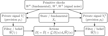
A two-player tracking game isolates the local feedback channel (Figure 1.1). Every figure in this section, and the solver behind it, runs in the browser at sbabichenko.com/noisestate with adjustable parameters.

1.2.1Primitives and objectives

Fix a horizon $[0, T]$ and a filtered probability space $(Ω, F, F, P)$ supporting a standard three-dimensional Brownian motion $W = (W^{0}, W^{1}, W^{2})$ , where $F = (F_{t})_{t \in [0, T]}$ is the completed, right-continuous natural filtration of $W$ . The state $X = (X_{t})_{t \in [0, T]}$ is the real-valued, ${F_{t}}$ -adapted process satisfying $d X_{t} = (D_{t}^{1} + D_{t}^{2}) d t + σ d W_{t}^{0}, X_{0} = x_{0}, (1.2.1)$ where $σ > 0$ is the fundamental volatility. Player $i \in {1, 2}$ does not observe $X$ directly; instead it observes the private diffusion channel $d Y_{t}^{1} = p_{1} X_{t} d t + d W_{t}^{1}, d Y_{t}^{2} = p_{2} X_{t} d t + d W_{t}^{2} . (1.2.2)$ The numbers $p_{i}$ are signal precisions. Player $i$ chooses $D^{i}$ using only its private observation history. Formally, $F^{i} = (F_{t}^{i})_{t \in [0, T]}$ is the completed, right-continuous augmentation of $σ (Y_{s}^{i} : 0 \leq s \leq t)$ , and an admissible control $D^{i}$ is $F^{i}$ -progressively measurable and square-integrable, $E \int_{0}^{T} (D_{t}^{i})^{2} d t < \infty$ . The two controls are adapted to different filtrations, $D^{1}$ to ${F_{t}^{1}}$ and $D^{2}$ to ${F_{t}^{2}}$ , and in general neither filtration contains the other.

Running costs are symmetric tracking losses with quadratic effort penalty $r > 0$ : $J^{1} (D^{1}; D^{2}) = E \int_{0}^{T} ((X_{t} - 1)^{2} + r (D_{t}^{1})^{2}) d t, J^{2} (D^{2}; D^{1}) = E \int_{0}^{T} ((X_{t} + 1)^{2} + r (D_{t}^{2})^{2}) d t . (1.2.3)$ Player 1 wants the state near $+ 1$ ; player 2 wants it near $- 1$ .

Each player minimizes its own cost, taking the opponent’s strategy as given. A pair $(D^{1 ⋆}, D^{2 ⋆})$ of admissible strategies is a Nash equilibrium if $J^{1} (D^{1 ⋆}; D^{2 ⋆}) \leq J^{1} (D^{1}; D^{2 ⋆})$ for every admissible $D^{1}$ , and symmetrically for player 2. Section 1.3.3 restates the definition for the $n$ -player game.

Figure 1.1. Information-to-action feedback in the worked example.

1.2.2Impulse responses and wedges

Equilibrium controls belong to the noise-state linear class (Definition 1.4) and can be written in two equivalent impulse-response coordinates, with the noise-state defined on the middle line: $D_{t}^{i} W_{t}^{i} (u) D_{t}^{i} = \overset{ˉ}{D}_{t}^{i} + \int_{0}^{t} D_{t}^{i} (u) d_{u} W_{t}^{i} (u), := E [W_{u} ∣ F_{t}^{i}], = \overset{ˉ}{D}_{t}^{i} + \int_{0}^{t} D_{W, t}^{i} (u) d W_{u} . (1.2.4)$ The first line is the strategy as the player implements it: a deterministic mean plus a reading of the noise-state. The third line is the same control composed with the player’s filter and written directly over the primitive shocks. $D_{t}^{i} (u)$ , the policy kernel, weights estimates measurable to the player, while $D_{W, t}^{i} (u)$ describes how the choice loads on the truth and involves every player’s filter.

Proposition 1.1 (Best responses and equilibrium in the two-player game). For every finite horizon and every fixed linear strategy of the opponent, each player has a unique best response over the full admissible class, and that response is noise-state linear. There is $T^{*} > 0$ such that for $T \leq T^{*}$ the game admits a noise-state linear equilibrium, unique in the strategy ball $B_{T}^{M_{0}}$ of Theorem A.7, Picard iteration converges to it geometrically, and the equilibrium is Nash over the full admissible class. For an arbitrary horizon, any strategy ball satisfying the weighted monotonicity and residual-radius conditions of Theorem A.9 contains a unique fixed point, and that fixed point is a Nash equilibrium over the full admissible class.

Proof. The coefficients are constant and bounded and the effort weights satisfy $r > 0$ , so Assumption A.1 (the boundedness and ellipticity conditions of Appendix A.2) holds. Apply Proposition 1.12, Theorem A.7, and Theorem A.9 with $n = 2$ and $d = 1$ . ◻

1.2.3The life of a spike deviation

A spike by one player propagates through the loop of Figure 1.1. Player 1 adds an impulse $z δ_{t}$ to its control. The state shifts by $z$ and stays shifted. Player 2’s innovation carries the part of the shift player 2 has not yet learned, $p_{2} (δ X_{τ} - δ X_{τ}^{2}) d τ$ , and each coordinate of its noise-state moves through the unresolved response, $X^{2}$ , the part of the shock’s effect player 2 has not yet resolved, $\partial_{τ} δ w_{τ}^{2} (u) = p_{2} X_{τ}^{2} (u) (δ X_{τ} - δ X_{τ}^{2}), δ X_{τ}^{2} = \int_{0}^{τ} X_{τ} (s) δ w_{τ}^{2} (s) d s,$ with the coordinate born at $τ$ equal to $p_{2} (δ X_{τ} - δ X_{τ}^{2})$ . Player 2’s control moves with its coordinates and the state with the control. Player 2’s target is $- 1$ , so the response opposes the shift.

Player 1 pays for the shift and for the response. The shift is priced at the running cost. The response is priced through player 2’s noise-state, one coordinate at a time: $H_{t}^{2, 1} (u)$ of (1.4.8), the belief price, is the marginal cost to player 1 of having moved player 2’s estimate of the shock at $u$ . Setting the variation to zero for every $F_{t}^{1}$ -measurable $z$ ,

$2 r D_{t}^{1} = - E [\int_{t}^{T} (2 (X_{τ} - 1) + V_{τ}^{1}) d τ F_{t}^{1}], V_{τ}^{1} = p_{2} E^{2} H_{τ}^{2, 1} (τ) + p_{2} \int_{0}^{τ} X_{τ}^{2} (v) H_{τ}^{2, 1} (v) d v, (1.2.5)$

which is (1.4.7) integrated, with the wedge (1.4.9) at the example’s coefficients. Without player 2 only the running-cost term $2 (X_{τ} - 1)$ remains; $V^{1}$ is the change in player 2’s beliefs times their price. Theorem 1.8 is the same calculation for $n$ players, a vector state, and a general observation map.

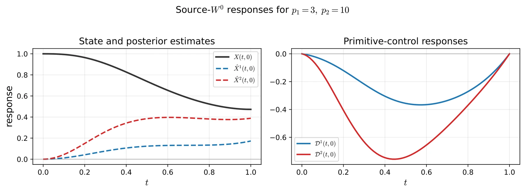
Player 2 sees the state only through its signal, so it cannot tell a unit spike by player 1 from a fundamental shock $d W^{0}$ of size $1/ σ$ . At $σ = 1$ , player 2’s curves in Figure 1.2 therefore show how player 2 responds to a unit spike by player 1. The left panel traces a single state shock through the actual state and through each player’s posterior estimate of it, each a linear readout of the game’s Markov state (the physical state together with every player’s noise-state; Section 1.3). The shock moves the state. Each player’s estimate catches up at a speed set by its signal precision. The right panel traces the same shock through the players’ actions. Each player responds to the shock through what it has learned, the better-informed player earlier and more strongly. Both control responses die out at the horizon, when nothing remains to be gained from moving the state. These plots can be redrawn at any parameters in the browser version.

Figure 1.2. Impulse responses to the first state shock $d W_{0}^{0}$ with $p_{1} = 3$ , $p_{2} = 10$ , and $r_{1} = r_{2} = 0.1$ . Left: state and posterior-estimate responses. Right: primitive-control responses $D_{W, t}^{1} (0)$ and $D_{W, t}^{2} (0)$ .

1.2.4Computation

The unknowns of the fixed point are the kernels $D_{t}^{i} (u)$ , $X_{t} (u)$ , and $F_{t}^{i} (u, s)$ ; the adjoint equations (1.4.7)–(1.4.8) are solved for these kernels rather than for a value function on $X_{t}$ , because each player’s response depends on every opponent’s filter. Equilibrium is computed as a fixed point of the simultaneous best-response map on the deterministic causal policy kernels, discretized on a uniform grid of $N = 40$ points; no Monte Carlo simulation is used. Starting from zero policy kernels, each outer iteration first solves the forward state–filter system generated by the current profile, then solves both players’ backward physical and belief-price equations, and finally applies the first-order conditions to obtain a new pair of policy kernels. Both new kernels come from the same old profile, so the update is simultaneous rather than alternating.

Write $G (D)$ for this discretized best-response map and $D = (D^{1}, D^{2})$ . Convergence is measured by the normalized Frobenius residual over every time pair on the discrete causal triangle and every primitive-shock coordinate, $resid (D) = \frac{∥ G ( D ) - D ∥ _{F}}{max { 1 , ∥ G ( D ) ∥ _{F} }} .$ The first update is a relaxed Picard step with relaxation parameter $0.15$ ; subsequent updates use depth-five Anderson acceleration with mixing parameter $0.6$ . The algorithm stops when the residual falls below $1 0^{- 5}$ . Within each outer iteration, the coupled forward state–filter calculation uses two relaxed updates of the state impulse response and six filter sub-iterations. After the policy kernels converge, a separate relaxed fixed-point iteration, initialized at zero and solved to tolerance $1 0^{- 10}$ , gives the deterministic mean controls and mean state. Parameter sweeps may be warm-started from the equilibrium at a neighboring parameter value.

Unless otherwise stated, $T = 1$ , $x_{0} = 0$ , $r = 0.1$ , $σ = 1$ , and there is no terminal cost. In an optimized native C++ build with OpenMP, the symmetric benchmark $(p_{1}, p_{2}) = (3, 3)$ at $N = 40$ converges in $42$ outer iterations and takes about $0.03$ seconds; at $N = 160$ the same benchmark takes about $1.4$ seconds.

The scheme is first order in the grid spacing. On the symmetric benchmark with targets $(1, - 1)$ , player 1’s cost is $4.219$ , $4.160$ , and $4.131$ at $N = 40$ , $80$ , and $160$ , an observed order of $1.06$ ; the policy kernels converge at the same rate. A single $N = 40$ run is therefore accurate to about 3 percent on costs and mean actions, and considerably worse on quantities small early in the horizon, such as the posterior estimates just after a shock and the information wedges. Unless a caption says spectral solution, figures and reported values below are Richardson extrapolations from two nested grids, $2 f_{157} - f_{79}$ , which agree with the extrapolation from $N = 40$ and $N = 79$ to within 0.3 percent except at the first two grid points of the wedge curves.

The solvers and figures of this section are the work of Claude Fable 5, a large language model built by Anthropic [7], working under the author’s direction. The interactive version at sbabichenko.com/noisestate runs the same solver.

1.2.5Mean actions, separation failure, and the welfare cost of belief manipulation

Since the stochastic integral in the first line of (1.2.4) has zero unconditional mean, $E [D_{t}^{i}] = \overset{ˉ}{D}_{t}^{i}$ isolates the deterministic tug-of-war over the target $\pm 1$ , while the response term captures impulse responses to posterior shocks.

Separation failure.

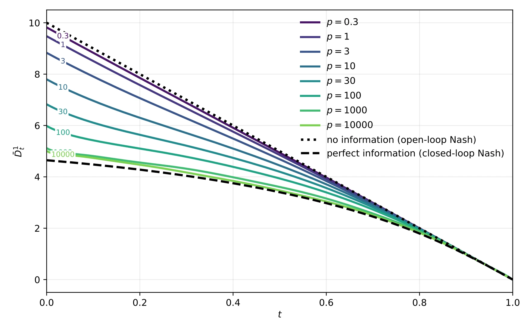
Under perfect information, the mean policy is independent of signal precision. Decentralized information breaks this. Changing signal precision changes how much of each shock remains unresolved for the opponent, which changes the belief price, so the policy rule moves independently of the state estimate (Remark 1.13). The mechanism is the information wedge.

Figure 1.3 plots the resulting failure. The equilibrium mean control path $\overset{ˉ}{D}_{t}^{1}$ shifts with the signal precision $p$ , and the partial-information paths lie between two limits independent of $p$ . With no information the players cannot see each other and the mean paths are the open-loop Nash equilibrium of the deterministic game, $\overset{ˉ}{D}_{t}^{1} = (T - t) / r$ . With perfect information they are its closed-loop Nash equilibrium, in which each player’s feedback on the state is priced by the other. As $p$ rises the mean control moves monotonically from the first to the second, and at $p = 1 0^{3}$ it is still ten percent above the closed-loop path, and at $p = 1 0^{4}$ seven percent. Under a separation principle the colored paths would sit on the closed-loop line at every precision. With $p_{1} = p_{2}$ , opposite targets, and $x_{0} = 0$ , the two mean controls cancel and $\overset{ˉ}{X}_{t} \equiv 0$ at every precision. The movement in Figure 1.3 is effort spent holding a path that does not change. It vanishes in models where information and incentives can be treated separately. Because the shift is in the mean $\overset{ˉ}{D}_{t}^{1}$ rather than in the zero-mean response term, it does not cancel when many independent copies of the market are averaged; Chapter 5 works this out.

Figure 1.3. Equilibrium mean control $\overset{ˉ}{D}_{t}^{1}$ as signal precision $p$ varies (spectral solution, both players at precision $p$ ). Dotted: the open-loop Nash path of the deterministic game, the no-information limit. Dashed: the closed-loop Nash path of the perfect-information game.

Information pooling as a corrective intervention.

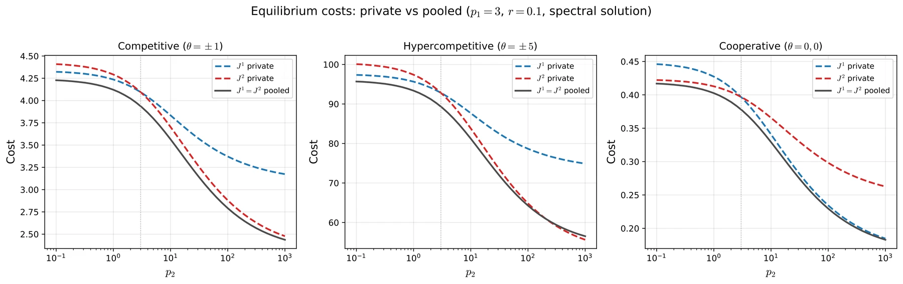
Figure 1.4 compares private signals with a pooled signal of precision $p_{1} + p_{2}$ under opposing targets $(\pm 1)$ and $(\pm 5)$ and a common target $(0)$ . At $(\pm 1)$ and $(0)$ pooling is Pareto-improving at every $p_{2}$ , and the gain is an order of magnitude larger under competition. Since the target change affects only the deterministic mean system, the common-target case isolates the pure estimation benefit. Each player still pays its own effort cost, so this case is a Nash game rather than the team problem of Section 1.4.1. The excess gain under competition is the welfare cost of bilateral belief manipulation.

The private-signal curves also show who wants the precision. Under the common target the better-informed player has the higher cost. At $p_{2} = 10$ player 2 pays $0.366$ against player 1’s $0.341$ . The better-informed player does more of the work, so each player would rather be the less precise one. Under opposing targets the ordering reverses, $3.70$ against $3.83$ , and precision is an advantage over the opponent. In absolute terms, both players gain when either one is better informed, including player 1, whose own precision is fixed and whose opponent improves. The competitive case does not change that even though it raises every cost by an order of magnitude. At $p_{2} = 1000$ the pooled cost and player 2’s private cost have nearly met, since a player who observes the state almost exactly has little left to learn from a pooled signal. With stronger conflict they cross. The policy kernels do not depend on the targets, and the mean paths are linear in them, so at targets $(k, - k)$ the cost is $J^{i} = J_{var}^{i} + k^{2} \overset{ˉ}{J}^{i}$ , with $J_{var}^{i}$ the cost at the common target and $\overset{ˉ}{J}^{i}$ the mean part at $(1, - 1)$ . Pooling still lowers player 2’s variance cost, but it raises its mean cost, because player 2 gives up the mean-path advantage of being the better informed. Above $p_{2} \approx 250$ the second effect wins. Pooling then costs player 2 ( $0.9$ at $p_{2} = 1000$ ) while player 1 gains $18$ . Under strong conflict the better-informed player prefers to keep its edge. Under the common target player 1’s private cost meets the pooled cost too ( $0.185$ against $0.183$ ), so an almost perfectly informed teammate is nearly as good as a shared signal. Under opposing targets it stays well above ( $3.17$ against $2.44$ ). An almost perfectly informed opponent is not.

Figure 1.4. Equilibrium costs under private signals (dashed) and a pooled signal (solid), with $p_{1} = 3$ fixed and $p_{2}$ varying from $0.1$ to $1000$ on a logarithmic axis (spectral solution). Left: opposing targets $(\pm 1)$ . Center: opposing targets $(\pm 5)$ . Right: common target $(0)$ . The vertical scales differ: costs are about $4$ , $80$ , and $0.4$ in the three panels, since the mean part of the cost scales with the square of the target. The dotted line marks $p_{2} = p_{1}$ .

1.2.6Optimal precision allocation

Information pooling is blunt. A planner with a fixed precision budget must still choose how to split it between the two players.

Setup.

Retain the state dynamics (1.2.1) and observation channels (1.2.2) with opposing targets ( $\pm 1$ ), but allow asymmetric precisions $(p_{1}, p_{2})$ subject to $p_{1} + p_{2} = \overset{ˉ}{P}$ and asymmetric effort costs $(r_{1}, r_{2})$ with $r_{1} < r_{2}$ , so player 1 is the more efficient mover of the state. A planner chooses the split to minimize aggregate equilibrium cost; for each candidate allocation the solver of Section 1.2.4 computes the full equilibrium. Parameters: $\overset{ˉ}{P} = 20$ , $T = 1$ , with the fundamental volatility in (1.2.1) reduced to $σ = 0.5$ . Because the players have opposing targets, their mean controls push in opposite directions rather than jointly stabilizing the state. Total destructive effort measures the intensity of this arms race, $E^{dest} = \int_{0}^{T} (r_{1} (E [D_{t}^{1}])^{2} + r_{2} (E [D_{t}^{2}])^{2}) d t .$

Figure 1.5. Equilibrium quantities across the precision split, $p_{1} + p_{2} = \overset{ˉ}{P} = 20$ , with opposing targets, $σ = 0.5$ , and asymmetric effort costs $(r_{1}, r_{2}) = (0.05, 0.2)$ . Left: individual costs. Center: total destructive effort (the aggregate quadratic cost of the mean controls). Right: mean controls and mean state.

Information starvation.

Under cooperation, a planner should assign precision to the efficient mover. Under competition, the natural guess is instead that a planner should balance precision to limit manipulation. Figure 1.5 shows the opposite. With asymmetric effort costs $(r_{1}, r_{2}) = (0.05, 0.2)$ , concentrating precision on the efficient player shifts the mean state toward that player’s target and sharply reduces destructive effort. On net, both players’ costs fall as destructive effort moves toward the perfect-information benchmark.

Denying the inefficient player signal access weakens the bilateral arms race: commitment in the sense of Schelling [105]. Giving all precision to the inefficient player produces the worst outcome, because the efficient player pushes hard against a well-informed opponent. The planner’s optimum is not balanced precision but an information monopoly for the efficient player. The right panel shows separation failure again. Certainty-equivalent controls are invariant to the split, while equilibrium controls move with the belief prices.

1.3The decentralized LQG game

Informal description of the game.

The games here have a common evolving state, private noisy observation channels, and controls that feed back into the state and so into others’ signals. These features generate the Townsend hierarchy of forecasting the forecasts of others [104, 109]; quadratic objectives and linear-Gaussian primitives make the problem tractable. The section generalizes Section 1.2: the same noise-state coordinates, filters, and prices, now with $n$ players, vector states, and general linear dynamics.

1.3.1State dynamics and objectives

Consider $n$ players interacting over a finite horizon $[0, T]$ on a filtered probability space $(Ω, F, F, P)$ .

State dynamics.

The state $X_{t} \in R^{d}$ evolves as $d X_{t} = (B_{X}^{X} (t) X_{t} + i = 1 \sum n B_{i}^{X} (t) D_{t}^{i}) d t + σ (t) d W_{t}^{0}, X_{0} = x_{0}, (1.3.1)$ where $B_{X}^{X} (t) \in R^{d \times d}$ is deterministic and bounded, $W^{0}$ is a $d$ -dimensional Brownian motion, $σ (t) \in R^{d \times d}$ is deterministic and bounded, and $D_{t}^{i} \in R^{d}$ is player $i$ ’s control, entering through the deterministic, bounded gain $B_{i}^{X} (t) \in R^{d \times d}$ (the identity in the examples).

Objectives.

Let $G_{t}^{X, i}$ denote the linear state-cost coefficient. In the baseline case it is deterministic and bounded.¹ Each player $i$ incurs the cost

$C^{i} (D^{i}; D^{- i}) := \frac{1}{2} \int_{0}^{T} (X_{t}^{⊤} G^{XX, i} (t) X_{t} + 2 (G_{t}^{X, i})^{⊤} X_{t} + 2 (D_{t}^{i})^{⊤} G^{D X, i} (t) X_{t} + (D_{t}^{i})^{⊤} G^{DD, i} (t) D_{t}^{i}) d t + \frac{1}{2} (X_{T}^{⊤} G^{XX, i} (T) X_{T} + 2 (G_{T}^{X, i})^{⊤} X_{T}), (1.3.2)$

where the joint running Hessian $(G^{XX, i} (t) G^{D X, i} (t) G^{X D, i} (t) G^{DD, i} (t))$ , with $G^{X D, i} = (G^{D X, i})^{⊤}$ , is symmetric positive semidefinite, $G^{DD, i} (t)$ and $G^{XX, i} (T)$ are positive semidefinite, and $D^{- i} := (D^{j})_{j \neq = i}$ denotes opponents’ controls. Control coercivity needs the Schur complement $S^{i} (t) := G^{DD, i} (t) - G^{D X, i} (t) (G^{XX, i} (t))^{+} G^{X D, i} (t) ⪰ λ I, λ > 0, (1.3.3)$ rather than $G^{DD, i} ⪰ λ I$ , which permits the form $(x - d)^{2}$ . Semidefiniteness gives $range G^{X D, i} \subseteq range G^{XX, i}$ , so the pseudo-inverse term is exact. The cross term $G^{D X, i}$ lets the price of the control depend on the state (an input bill paid at a market price, a trading profit $D_{t}^{i} (V_{t} - P_{t})$ ); $G^{D X, i} \equiv 0$ is the tracking case, where $S^{i} = G^{DD, i}$ . Each player $i$ seeks to minimize $J^{i} (D^{i}; D^{- i}) := E [C^{i} (D^{i}; D^{- i})] . (1.3.4)$ Opponents’ controls enter player $i$ ’s cost only through $X_{t}$ , which they move through (1.3.1) and which player $i$ observes through (1.3.5).

1.3.2Information structure

Observations.

Player $i$ does not observe $X_{t}$ directly. Instead, its private information comes through the diffusion signal

$d Y_{t}^{i} = B_{X}^{Y, i} (t) X_{t} d t + E^{i} d W_{t}, Y_{0}^{i} = 0, (1.3.5)$ where $B_{X}^{Y, i} (t) \in R^{d \times d}$ is a deterministic observation gain and $E^{i} \in R^{d \times (n + 1) d}$ is the block selector extracting player $i$ ’s noise channel ( $W_{t}^{i} := E^{i} W_{t}$ ). All Brownian motions ${W^{0}, W^{1}, \dots, W^{n}}$ are mutually independent. The precision matrix $P^{i} (t) := B_{X}^{Y, i} (t)^{⊤} B_{X}^{Y, i} (t)$ measures the Fisher information about the state per unit time. The block-selector form is without loss, since replacing $E^{i}$ by a general invertible noise loading $σ^{i} (t)$ substitutes $(B_{X}^{Y, i})^{⊤} (σ^{i} σ^{i, ⊤})^{- 1}$ for $(B_{X}^{Y, i})^{⊤}$ everywhere. Throughout the main characterization, the gain $B_{X}^{Y, i} (\cdot)$ is fixed; the two-player benchmark studies comparative statics and planner-chosen precision.

Notation for primitive shocks.

Collect all primitive shocks into a single vector $W_{t} := (W_{t}^{0}, \dots, W_{t}^{n})^{⊤} \in R^{(n + 1) d}$ . The direct projection $Π^{i} := E^{i, ⊤} E^{i}$ is the identity on the $i$ -th block and zero elsewhere. The block-selector structure ensures each player’s observation noise is an independent component of $W$ . Player $i$ observes $Π^{i} W$ directly up to a drift term and infers $(I - Π^{i}) W$ from drift-based learning (Theorem 1.5).

Player $i$ ’s information at time $t$ is its observation history, $F_{t}^{i} := σ (Y_{s}^{i} : s \leq t)$ . An admissible control is $F_{t}^{i}$ -adapted with $E [\int_{0}^{T} ∥ D_{t}^{i} ∥^{2} d t] < \infty$ , where $∥ \cdot ∥$ denotes the Euclidean norm on $R^{d}$ .

Unresolved response.

For each player $i$ , define $X_{t}^{i} (u) := X_{t} (u) - X_{t}^{i} (u),$ the component of the state’s impulse response to the $u$ -th shock that player $i$ has not yet resolved at time $t$ . It is large when the shock is recent or the observation channel weak, and it shrinks as observations accumulate. Formally, $X_{t}^{i} (u) = Cov (X_{t}, d W_{u} ∣ F_{t}^{i}) / d u$ ; it is the filtering gain in the noise-state update (Theorem 1.5), with its explicit formula in (1.A.4).

1.3.3Nash equilibrium

Each player’s drift depends on opponents’ estimates $X_{t}^{k} := E [X_{t} ∣ F_{t}^{k}]$ . The following equilibrium concept fixes opponents’ strategy maps rather than their realized actions; Section 1.4 needs this to show that a best response to noise-state linear opponents is itself noise-state linear.

Definition 1.2 (Nash equilibrium in private-signal strategies). Throughout, a player’s choice is a strategy map: for each $t \in [0, T]$ , the action $D_{t}^{i}$ is a (progressively measurable) functional of the private observation history $Y_{\cdot\land t}^{i}$ . Write $D_{t}^{i} = D_{t}^{i} [Y^{i}]$ , where the bracket notation $D_{t}^{i} [\cdot]$ denotes the map from the observation path $(Y_{s}^{i})_{s \leq t}$ to the action at time $t$ . Admissible strategy maps must satisfy $E \int_{0}^{T} ∥ D_{t}^{i} ∥^{2} d t < \infty$ and must also be causally well posed: against any fixed profile of the opponents’ complete causal maps, the coupled state–observation–strategy equations admit a unique strong causal solution, adapted to the control-free observation filtration. Strategies use no independent randomization; any private randomization, if admitted, is included in the player’s filtration.

A profile $D^{*} = (D^{*, 1}, \dots, D^{*, n})$ is a Nash equilibrium if for every player $i$ and every admissible alternative strategy map $D^{i} [\cdot]$ , $J^{i} (D^{*, i}; D^{*, - i}) \leq J^{i} (D^{i}; D^{*, - i}) .$

Holding opponents’ strategy maps fixed is substantive because signals are endogenous. A unilateral deviation changes the drifts of opponents’ observation paths, and with them the likelihoods they assign to histories. Under admissible square-integrable controls this only changes drifts, so the induced observation laws are mutually absolutely continuous on every finite horizon. A perfect-Bayesian formulation is simpler here than in discrete signal games, because Bayes’ rule applies on a common support and the fixed strategy maps are evaluated on whatever observation paths occur.

Noise-state.

On a given profile, the noise-state is the conditional mean path of the aggregated primitive shock: $W_{t}^{i} (u) := E [W_{u} ∣ F_{t}^{i}], 0 \leq u \leq t . (1.3.6)$ Against fixed opponent maps, player $i$ ’s realized control is a known input. Proposition 1.6 shows that its full downstream effect on the state, on opponents’ responses, and so on $Y^{i}$ is a deterministic causal functional of the realized control path. Subtracting that effect gives a control-free Gaussian observation with the same filtration. Off the candidate profile, $W^{i}$ then denotes the conditional projection of $W$ in this equivalent reference coordinate. The deviating player does not choose a filter. The actual conditional state estimate is the reference estimate plus the known state response, while the innovation and its covariance are unchanged. On the candidate profile this agrees with (1.3.6).

Definition 1.3 ((Primitive-shock) linear process). An $L^{2}$ stochastic process $L = (L_{t})_{t \in [0, T]}$ is a (primitive-shock) linear process if there exist deterministic functions $\overset{ˉ}{L} : [0, T] \to R^{m}, L : [0, T]^{2} \to R^{m \times (n + 1) d},$ such that, for every $t \in [0, T]$ , $L_{t} = \overset{ˉ}{L} (t) + \int_{0}^{t} L (t, s) d W_{s}, \int_{0}^{t} ∥ L (t, s) ∥^{2} d s < \infty.$ When convenient, extend $L (t, s)$ by $0$ for $s > t$ .

Definition 1.4 (Noise-state linear control / strategy). An admissible strategy map is noise-state linear if, for the fixed filter described above, there exist deterministic functions $\overset{ˉ}{D}^{i} : [0, T] \to R^{d}, D^{i} : [0, T]^{2} \to R^{d \times (n + 1) d},$ such that, for every private history $Y^{i}$ and every $t \in [0, T]$ , $D_{t}^{i} [Y^{i}] = \overset{ˉ}{D}_{t}^{i} + \int_{0}^{t} D_{t}^{i} (u) d_{u} W_{t}^{i} [Y^{i}] (u), \int_{0}^{t} ∥ D_{t}^{i} (u) ∥^{2} d u < \infty.$ Extend $D_{t}^{i} (u)$ by $0$ for $u > t$ and drop the argument $[Y^{i}]$ on the equilibrium path.

1.4General theory

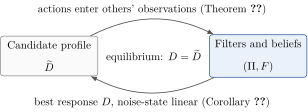
The primitive-shock space plays the role of a dynamic Harsanyi type space [52]: conditional beliefs are projections of $W = (W^{0}, \dots, W^{n})$ onto private signal histories. Higher-order beliefs are compositions of these projections. Player $i$ ’s estimate of player $k$ ’s estimate of the state is $E [X_{t}^{k} ∣ F_{t}^{i}]$ ; since $X_{t}^{k}$ is a linear functional of $d W_{t}^{k}$ with the deterministic state kernel $X_{t} (\cdot)$ , its projection onto $F_{t}^{i}$ is the same functional applied to $E [d_{s} W_{t}^{k} (s) ∣ F_{t}^{i}]$ , which is (1.4.1) for player $k$ evaluated on player $i$ ’s noise-state. Every order of belief is therefore a finite composition of the kernels $(Π^{k}, F^{k})$ , and no new state variable is needed. Actions reshape the signals from which beliefs are formed, so those maps must be solved as a fixed point (Figure 1.6).

Figure 1.6. Noise-state fixed-point loop. Each map determines the other, so the profile must be solved as a fixed point.

Beliefs as deterministic kernels.

The noise-state $W_{t}^{i} (\cdot)$ of (1.3.6) has a deterministic-kernel representation for its estimated-noise increments on the causal triangle $Δ_{T} = {(t, s) : 0 \leq s \leq t \leq T}$ , extended by zero off $Δ_{T}$ . Write $d_{u}$ for increments in the path index (the source time $u$ ) and $d_{t}$ for updates in time. The state has the form $X_{t} = \overset{ˉ}{X}_{t} + \int_{0}^{t} X_{t} (s) d W_{s}$ , with $X_{t} (s)$ the impulse-response kernel. Appendix 1.A gives the general linear-filtering result; here $C (t, s) = B_{X}^{Y, i} (t) X_{t} (s)$ .

Theorem 1.5 (Beliefs are deterministic kernels: Filtering Closure). Fix a player $i$ . Assume the state admits the primitive-shock linear form $X_{t} = \overset{ˉ}{X}_{t} + \int_{0}^{t} X_{t} (s) d W_{s},$ and player $i$ observes $d Y_{t}^{i} = B_{X}^{Y, i} (t) X_{t} d t + E^{i} d W_{t},$ with deterministic $P^{i} (t) ⪰ 0$ and block selector $E^{i}$ .

Let $Π^{i} := E^{i, ⊤} E^{i}$ and $X_{t}^{i} := E [X_{t} ∣ F_{t}^{i}]$ , and define the innovation $d I_{t}^{i} := d Y_{t}^{i} - B_{X}^{Y, i} (t) X_{t}^{i} d t$ .

(i) The estimated-noise path increments admit the decomposition $d_{u} W_{t}^{i} (u) = directly observed Π^{i} d W_{u} + indirect inference (\int_{0}^{t} F_{t}^{i} (u, s) d W_{s}) d u, u < t, (1.4.1)$ where the deterministic kernel $F^{i}$ is given by $F_{t}^{i} (u, s) = X_{s}^{i} (u)^{⊤} B_{X}^{Y, i} (s)^{⊤} E^{i} + E^{i, ⊤} B_{X}^{Y, i} (u) X_{u}^{i} (s) + \int_{m a x (u, s)}^{t} X_{r}^{i} (u)^{⊤} P^{i} (r) X_{r}^{i} (s) d r . (1.4.2)$ The pair $(Π^{i}, F^{i})$ is the blueprint of player $i$ ’s beliefs.

(ii) The mixed $(t, u)$ -update satisfies $d_{t} (d_{u} W_{t}^{i} (u)) = X_{t}^{i} (u)^{⊤} B_{X}^{Y, i} (t)^{⊤} d I_{t}^{i} d u .$ Each old coordinate moves with the innovation, and $X_{t}^{i} (u)$ is the gain. The singular term $Π^{i} d W_{t}$ is the coordinate’s birth, its entry into the filter at the current date.

The unresolved response $X^{i}$ is determined algebraically from $F^{i}$ by (1.A.4); the filter kernel $F^{i}$ is the unique solution of the forward evolution system (1.A.5)–(1.A.6) (Definition 1.16).

Proposition 1.6 (Against frozen opponents, the deviating player’s own control is a known input to its filter). Fix player $i$ and the opponents’ complete noise-state linear strategy maps, including their filters. Let $D^{i}$ and $D^{i}$ be any two admissible controls generated by causally well-posed strategy maps, and write $Δ D^{i} := D^{i} - D^{i}, Δ X := X^{D^{i}} - X^{D^{i}} .$ The corresponding differences in the state, opponents’ noise-states, and opponents’ controls satisfy the exact deterministic causal system stated in (1.B.1)–(1.B.3). That system is linear in the realized input process $Δ D^{i}$ even when the feedback rule generating $D^{i}$ is nonlinear. No small-deviation approximation is used.

The own-observation difference is $d Y_{t}^{i, D^{i}} - d Y_{t}^{i, D^{i}} = B_{X}^{Y, i} (t) Δ X_{t} d t, (1.4.3)$ and $Δ X_{t}$ is a deterministic causal functional of $Δ D_{[0, t]}^{i}$ . Taking $D^{i} \equiv 0$ , define the control-free (reference) observation by subtracting this known response from the actual observation. Causal well-posedness gives an invertible causal correspondence between the actual and control-free histories, so they generate the same completed filtration. If $X^{i, 0}$ and $Y^{i, 0}$ denote the control-free state and observation, then $d I_{t}^{i} := d Y_{t}^{i, 0} - B_{X}^{Y, i} (t) X_{t}^{i, 0} d t = d Y_{t}^{i, D^{i}} - B_{X}^{Y, i} (t) (X_{t}^{i, 0} + Δ X_{t} [D^{i}]) d t (1.4.4)$ is the same standard Brownian innovation under every admissible strategy of player $i$ . The deviating player’s filter is then the conditional filter implied by the frozen environment and the known input.

Lemma 1.7 (Noise-state integrals as innovation integrals). Fix $t$ and let $K_{t} : [0, t] \to R^{m \times (n + 1) d}$ be deterministic and square-integrable. In the reference innovation coordinate of Proposition 1.6, $\int_{0}^{t} K_{t} (u) d_{u} W_{t}^{i} (u) = \int_{0}^{t} [K_{t} (s) E^{i, ⊤} + \int_{0}^{s} K_{t} (u) X_{s}^{i} (u)^{⊤} B_{X}^{Y, i} (s)^{⊤} d u] d I_{s}^{i} . (1.4.5)$ The closed linear span of the coordinates ${W_{t}^{i} (u) : 0 \leq u \leq t}$ contains every $F_{t}^{i}$ -measurable affine Gaussian random variable, so each has a deterministic noise-state representation. Equation (1.4.5) gives the corresponding innovation coefficient.

Proof. Integrating the mixed update in Theorem 1.5 from the birth time $u$ to $t$ gives, as a measure in $u$ , $d_{u} W_{t}^{i} (u) = E^{i, ⊤} d I_{u}^{i} + (\int_{u}^{t} X_{s}^{i} (u)^{⊤} B_{X}^{Y, i} (s)^{⊤} d I_{s}^{i}) d u .$ Substitution followed by stochastic Fubini gives (1.4.5). For the span claim, conditional expectation is the orthogonal projection of linear functionals of the primitive shock onto the $F_{t}^{i}$ -measurable ones. The projected primitive increments $d_{u} W_{t}^{i} (u) = E [d W_{u} ∣ F_{t}^{i}]$ then generate precisely that subspace. ◻

Best-response verification and information wedges.

The maximum-principle calculation identifies deterministic adjoint kernels and the information wedge $V^{i} (t)$ . The exact finite-deviation identity below then verifies the resulting candidate against the full admissible $L^{2}$ class.

Theorem 1.8 (Belief prices and information wedges). Fix a player $i$ and suppose each opponent $k \neq = i$ uses a noise-state linear strategy with deterministic impulse-response maps, which pins down a deterministic forward environment (state impulse response $X (\cdot, \cdot)$ , filtering objects $(P^{k}, X^{k}, F^{k})$ , and policy kernels $D^{k}$ ). There exist linear processes $H_{t}^{X, i}$ and $H_{t}^{k, i} (u)$ , $k \neq = i$ , such that the following system holds for $t \in [0, T]$ , with (1.4.8) holding for old-history coordinates $0 \leq u < t$ . For each opponent $k \neq = i$ , define $V_{t}^{k, i} := B_{X}^{Y, k} (t)^{⊤} E^{k} H_{t}^{k, i} (t) + P^{k} (t) \int_{0}^{t} X_{t}^{k} (r) H_{t}^{k, i} (r) d r, V_{t}^{i} := k \neq = i \sum V_{t}^{k, i} . (1.4.6)$ The state price and belief prices satisfy $\frac{d}{d t} H_{t}^{X, i} \frac{d}{d t} H_{t}^{k, i} (u) = perfect-information costate block [- (G^{XX, i} (t) X_{t} + G_{t}^{X, i} + G^{X D, i} (t) D_{t}^{i}) - B_{X}^{X} (t)^{⊤} H_{t}^{X, i}] - information wedge V_{t}^{i}, = - (B_{k}^{X} (t) D_{t}^{k} (u))^{⊤} H_{t}^{X, i} + X_{t} (u)^{⊤} V_{t}^{k, i}, k \neq = i, (1.4.7) (1.4.8)$ with terminal conditions $H_{T}^{X, i} = G^{XX, i} (T) X_{T} + G_{T}^{X, i}$ and $H_{T}^{k, i} (\cdot) = 0$ . All coefficients, $P^{k} (t)$ , $X_{t}^{k} (r)$ , $D_{t}^{k} (u)$ , and $X_{t} (u)$ , are determined by opponents’ frozen strategy maps and do not change when player $i$ deviates.

Proof. Appendix 1.B.2: the spike variation, the opponent filter variation, the coupled state–filter system, and the backward adjoints. The state price $H_{t}^{X, i}$ is the marginal cost of a spike that moves the state at $t$ , and $H_{t}^{k, i} (u)$ the marginal cost of one that moves opponent $k$ ’s estimate of the shock at $u$ . Every channel through which player $i$ ’s action moves what opponents believe, and every consequence of those moved beliefs, enters the dynamics of the state price only through the term $V_{t}^{i}$ in (1.4.7). To write $V_{t}^{k, i}$ explicitly, define the filter contraction of a kernel $M (r)$ , $0 \leq r \leq t$ , and its transpose action on a row-valued kernel $N (r)$ by $B^{k} M := E^{k} M (t) + \int_{0}^{t} C_{t}^{k, Y} (r) M (r) d r, N B^{k ⊤} := N (t) E^{k ⊤} + \int_{0}^{t} N (r) C_{t}^{k, Y} (r)^{⊤} d r, (1.4.9)$ with $C_{t}^{k, Y} (r) = B_{X}^{Y, k} (t) X_{t}^{k} (r)$ . Then $V_{t}^{k, i} = B_{X}^{Y, k} (t)^{⊤} B^{k} H_{t}^{k, i}$ . The contraction $B^{k} H$ of (1.4.9) is opponent $k$ ’s filter applied to a belief price: the birth term $E^{k} H (t)$ for the shock arriving now, plus the integral of $H$ against the innovation kernel $C_{t}^{k, Y}$ for the shocks already in the history. Chapters 2, 4, and 6 reuse it with $(E^{k}, C^{k, Y})$ replaced by each chapter’s observer pair. In (1.4.8), $- (B_{k}^{X} (t) D_{t}^{k} (u))^{⊤} H_{t}^{X, i}$ is what player $i$ pays, at the state price, for the action opponent $k$ takes on a moved coordinate.

For a fixed profile, the continuation value is a functional of the physical state and the players’ noise-states, with adjoints $H_{t}^{X, i} = \partial_{X} V_{t}^{i}$ and $H_{t}^{k, i} (u) = δ V_{t}^{i} / δ W_{t}^{k} (u)$ . All coefficients in (1.4.7)–(1.4.8) are deterministic, so the mean and response-map coefficients decouple.

Corollary 1.9 (No observational externality). Suppose the state components that opponents observe are unaffected by player $i$ ’s control. Then a unilateral deviation in $D^{i}$ leaves every opponent’s observation law, and hence the fixed filter for each $W^{k}$ , $k \neq = i$ , unchanged; $V_{t}^{i} \equiv 0$ , the belief-price equations (1.4.8) decouple from the state price, and the optimality system reduces to the standard LQG game with fixed information structures.

Conversely, a player can be made to ignore the effect of its own actions on the other players’ beliefs by setting its information wedge to zero, which is how the exogenous-signal benchmarks of the later chapters are constructed.

Lemma 1.10 (Strict convexity on the fixed reference filtration). Fix opponents’ complete causal maps, use the reference filtration of Proposition 1.6, and suppose the joint running Hessian is positive semidefinite and (1.3.3) holds. Then player $i$ ’s objective is strictly convex and coercive on the admissible $L^{2}$ control space. For any two controls the state difference is the exact linear causal response to their control difference, and the quadratic part of the cost difference is half the joint form in $(Δ X, Δ D^{i})$ , which is nonnegative and dominates $\frac{1}{2} λ E \int_{0}^{T} ∥Δ D_{t}^{i} ∥^{2} d t$ after completing the square in $Δ X$ .

Proof. Proposition 1.6 makes the state and all induced opponent responses affine functions of the realized own-control input on one fixed adapted Hilbert space. Substituting them, the running integrand is half the joint form in $(Δ X, Δ D^{i})$ ; completing the square in $Δ X$ leaves $(Δ D^{i})^{⊤} S^{i} Δ D^{i}$ plus a nonnegative $G^{XX, i}$ term, so (1.3.3) gives the claim. ◻

A candidate that solves the stationarity system is a best response against every admissible deviation, including those outside the linear class.

Corollary 1.11 (Exact finite-deviation identity and best response over the full admissible class: Best Response Closure). Under the conditions of Theorem 1.8 and the Schur condition (1.3.3), let $D^{i, *}$ be a noise-state linear candidate whose deterministic kernels satisfy the stationarity system (1.B.13), and let $H^{X, i, *}$ be the corresponding state price. For every admissible strategy map $D^{i}$ of any form, set $Δ D^{i} := D^{i} - D^{i, *}, Δ X := X^{D^{i}} - X^{D^{i, *}} .$ Then the following identity is exact:

$J^{i} (D^{i}; D^{- i}) - J^{i} (D^{i, *}; D^{- i}) = E \int_{0}^{T} (Δ D_{t}^{i})^{⊤} [G^{DD, i} (t) D_{t}^{i, *} + E [G^{D X, i} (t) X_{t}^{*} + B_{i}^{X} (t)^{⊤} H_{t}^{X, i, *} ∣ F_{t}^{i}]] d t + \frac{1}{2} E \int_{0}^{T} [(Δ X_{t})^{⊤} G^{XX, i} (t) Δ X_{t} + 2 (Δ D_{t}^{i})^{⊤} G^{D X, i} (t) Δ X_{t} + (Δ D_{t}^{i})^{⊤} G^{DD, i} (t) Δ D_{t}^{i}] d t + \frac{1}{2} E [(Δ X_{T})^{⊤} G^{XX, i} (T) Δ X_{T}] . (1.4.10)$

The kernel stationarity equations make the first line on the right vanish for every adapted finite deviation. $D^{i, *}$ is then the unique best response over the full admissible $L^{2}$ class.

Proof. Appendix 1.B derives (1.4.10) by applying the physical and belief prices to the exact finite-difference system. Stationarity gives $G^{DD, i} D^{i, *} + E [G^{D X, i} X^{*} + (B_{i}^{X})^{⊤} H^{X, i, *} ∣ F^{i}] = 0$ . The remaining terms are the joint quadratic form, nonnegative by Lemma 1.10, and bounded below by $\frac{1}{2} λ E \int_{0}^{T} ∥Δ D_{t}^{i} ∥^{2} d t$ after completing the square. ◻

Corollary 1.11 takes a solution of the stationarity equations as given; the next proposition shows the best response exists.

Proposition 1.12 (Global solvability of unilateral best responses). Fix a finite horizon $T$ and complete linear causal strategy maps for all opponents, including their fixed filters from observations to controls. Under Assumption A.1, player $i$ ’s optimization problem has a unique best response over the full admissible $L^{2}$ control class. By Corollary 1.11, this best response is noise-state linear.

The proof is in Appendix A.2.

Remark 1.13 (Separation and the information wedge). Standard LQG separation holds the feedback gain fixed as signal precision changes. Here the FOC, $D_{t}^{i} = - (G^{DD, i} (t))^{- 1} E [G^{D X, i} (t) X_{t} + B_{i}^{X} (t)^{⊤} H_{t}^{X, i} ∣ F_{t}^{i}]$ , depends on the player’s conditional expectation of the state price. When actions affect opponents’ signals, that state price contains the wedge, which depends on opponents’ filters and belief prices. Changing information then generally changes the policy rule itself, not only the posterior variance.

1.4.1Identical-interest LQG games with control externalities

The baseline decentralized LQG game lets opponents’ controls affect player $i$ ’s payoff only through the state $X_{t}$ . In the identical-interest variant, every player evaluates the same quadratic cost of the full control profile. The state and observation equations (1.3.1) and (1.3.5) are unchanged. Let $D_{t} := ((D_{t}^{1})^{⊤}, \dots, (D_{t}^{n})^{⊤})^{⊤} \in R^{n d} .$ Fix deterministic weights $Q (t) = Q (t)^{⊤} ⪰ 0, R (t) = R (t)^{⊤} ≻ 0, Q_{T} = Q_{T}^{⊤} ⪰ 0,$ together with deterministic linear terms $q_{t}$ and $q_{T}$ and a deterministic constant $c (t)$ . The common cost is $C^{coop} (D) := \frac{1}{2} \int_{0}^{T} [X_{t}^{⊤} Q (t) X_{t} + 2 q_{t}^{⊤} X_{t} + c (t) + D_{t}^{⊤} R (t) D_{t}] d t + \frac{1}{2} (X_{T}^{⊤} Q_{T} X_{T} + 2 q_{T}^{⊤} X_{T}) . (1.4.11)$ Every player has the same objective, $J^{i} (D^{i}; D^{- i}) := E [C^{coop} (D^{i}, D^{- i})], i = 1, \dots, n .$ A profile $D^{*}$ is a cooperative Nash equilibrium if, for every player $i$ and every admissible private-signal strategy $D^{i}$ , $E [C^{coop} (D^{*})] \leq E [C^{coop} (D^{i}, D^{*, - i})] .$ Any global solution of the decentralized team problem is a cooperative Nash equilibrium.

Identical-interest games with dispersed information are the team problem of Radner [97] and Marschak and Radner [82]; the common-information approach of Nayyar et al. [89] solves the case in which every player also observes a common signal history. Here the information structure remains decentralized: player $i$ still computes the best response in the filtration $F_{t}^{i}$ , and a unilateral deviation still propagates through the other players’ private filters. In the identical-interest case the wedge no longer prices an adversarial manipulation of beliefs.

The filtering equations are unchanged, since the observation system is unchanged. Only the source terms in the control first-order system change. Let $L_{X} (t) L_{D}^{k} (t) := Q (t) X_{t} + q_{t}, := the k -th d -dimensional block of L_{D} (t) . L_{D} (t) := R (t) D_{t},$ For player $i$ , the state price satisfies $\frac{d}{d t} H_{t}^{X, i} = - L_{X} (t) - B_{X}^{X} (t)^{⊤} H_{t}^{X, i} - V_{t}^{i}, H_{T}^{X, i} = Q_{T} X_{T} + q_{T} . (1.4.12)$

For each opponent $k \neq = i$ , the belief price becomes $\frac{d}{d t} H_{t}^{k, i} (u) = - (B_{k}^{X} (t) D_{t}^{k} (u))^{⊤} H_{t}^{X, i} - (D_{t}^{k} (u))^{⊤} L_{D}^{k} (t) + X_{t} (u)^{⊤} V_{t}^{k, i}, H_{T}^{k, i} (\cdot) = 0. (1.4.13)$ The information wedge is the same filtering chain-rule object as before, (1.4.6). The new source term $- (D_{t}^{k} (u))^{⊤} L_{D}^{k} (t)$ is the effort cost of the control opponent $k$ takes, through its future posterior, in response to player $i$ ’s deviation. Under the common objective, player $i$ pays that cost too.

The best-response first-order condition is $E [L_{D}^{i} (t) + B_{i}^{X} (t)^{⊤} H_{t}^{X, i} F_{t}^{i}] = 0. (1.4.14)$ Equivalently, writing the block decomposition $L_{D}^{i} (t) = R_{ii} (t) D_{t}^{i} + j \neq = i \sum R_{ij} (t) D_{t}^{j},$ and assuming $R_{ii} (t) ≻ 0$ , the cooperative Nash policy satisfies $D_{t}^{i} = - R_{ii} (t)^{- 1} E B_{i}^{X} (t)^{⊤} H_{t}^{X, i} + j \neq = i \sum R_{ij} (t) D_{t}^{j} F_{t}^{i} . (1.4.15)$ In the separable-effort case, $D_{t}^{⊤} R (t) D_{t} = j = 1 \sum n (D_{t}^{j})^{⊤} R_{j} (t) D_{t}^{j},$ this reduces to $D_{t}^{i} = - R_{i} (t)^{- 1} B_{i}^{X} (t)^{⊤} E [H_{t}^{X, i} ∣ F_{t}^{i}],$ but the opponent-effort terms still enter the belief-price equations through $- (D_{t}^{k} (u))^{⊤} R_{k} (t) D_{t}^{k}$ .

The objective remains quadratic and the state, filters, and frozen opponent maps remain linear in the unilateral best-response problem, so the best response is again noise-state linear. A fixed point of the resulting cooperative best-response system is then a Nash equilibrium in private-signal strategies with a common objective.

1.5Conclusion

In the continuous-time LQG benchmark, beliefs, prices, and policy kernels are deterministic impulse-response kernels. Corollary 1.11 verifies that a fixed point in the noise-state linear class is a Nash equilibrium against arbitrary admissible $L^{2}$ deviations. The two-player examples show that the wedge changes welfare comparisons, information design, and the response to signal precision. Even with identical interests, teammates’ effort enters the belief prices.

The following chapters keep the same objects and change the environment. Chapter 2 adds delayed observation rows, Chapter 3 rewrites the kernel system in stationary lag form, and Chapter 4 applies the adjoint logic to order-flow trading. Chapter 5 uses symmetry to solve finite local strategic-information games in relative-position coordinates, then aggregates their equilibrium outcomes across markets. Chapter 6 makes the observability of a deviation player-dependent.

Appendices to Chapter 1

The two appendices following Chapter 1 contain the canonical derivations used throughout the dissertation. Appendix 1.A derives the filtering closure and the primitive-noise representation of the noise state. Appendix 1.B derives the control first-order conditions, belief adjoints, and information wedge. Later chapters modify these objects rather than rederive them from scratch.

Proof-local notation.

The symbols this appendix introduces for test functions, filter errors, and characteristic-function arguments are local to the proof in which they appear.

1.AFiltering

Theorem 1.5 follows by specializing a generic linear-filtering result to the physical observation model and then converting from innovations to primitive-shock coordinates.

1.A.1Dynamics of the noise-state

Fix a player $i$ . Recall the noise-state $W_{t}^{i} (u) := E [W_{u} ∣ F_{t}^{i}]$ , $0 \leq u \leq t$ , and the observation channel $d Y_{t}^{i} = (\overset{ˉ}{C} (t) + \int_{0}^{t} C_{t} (s) d W_{s}) d t + E^{i} d W_{t}, Y_{0}^{i} = 0,$ where $C_{t} (s)$ is deterministic. Since $\overset{ˉ}{C}$ is deterministic, set $\overset{ˉ}{C} \equiv 0$ without loss by replacing $Y_{t}^{i}$ with $Y_{t}^{i} - \int_{0}^{t} \overset{ˉ}{C} (r) d r$ .

Standing notation. Write $i := - 1$ in bold (to distinguish it from the player index $i$ ) and $R := L^{\infty} ([0, t]; R^{d_{Y}})$ ; take all $L^{2}$ spaces to be complex; normalize the observation noise so that $E^{i} E^{i ⊤} = I_{d_{Y}}$ , so $d ⟨ Y^{i} ⟩_{t} = I_{d_{Y}} d t$ ; and assume $C (t, \cdot) \in L^{2} ([0, t]; R^{d_{Y} \times d_{W}})$ for each $t$ , so that $W_{t}^{i} (u) = E [W_{u} ∣ F_{t}^{i}] \in L^{2}$ .

Lemma 1.14 (Test functionals). For $λ \in R$ let $φ^{λ}$ solve $d φ_{s}^{λ} = i φ_{s}^{λ} (d Y_{s}^{i})^{⊤} λ (s), φ_{0}^{λ} = 1.$ Each $φ_{t}^{λ}$ is bounded, and ${φ_{t}^{λ} : λ \in R}$ is total in $L^{2} (F_{t}^{i})$ . Consequently an $F_{t}^{i}$ -adapted $L^{2}$ process equals $E [W_{u} ∣ F_{t}^{i}]$ if it matches the test integrals $E [\cdot φ_{t}^{λ}] = E [W_{u} φ_{t}^{λ}] for every λ \in R .$

Proof. Each $φ_{t}^{λ}$ is $F_{t}^{i}$ -measurable, and Itô’s formula with $d ⟨ Y^{i} ⟩_{s} = I_{d_{Y}} d s$ gives $d ∣ φ_{s}^{λ} ∣^{2} = ∣ φ_{s}^{λ} ∣^{2} ∣ λ (s) ∣^{2} d s$ ; so $∣ φ_{t}^{λ} ∣ = exp (\frac{1}{2} \int_{0}^{t} ∣ λ ∣^{2} d s)$ is deterministic and $φ_{t}^{λ}$ is bounded. For a Brownian motion the family is total by [14, Lemma B.39]. The drift $\int_{0}^{\cdot} C (\cdot, s) d W_{s}$ of $Y^{i}$ is square-integrable, so $Law (Y^{i}) ≪ Law (β)$ for the Brownian motion $β$ with the same diffusion coefficient (Girsanov), with density $Λ$ . Totality transfers. If $E [Z φ_{t}^{λ}] = 0$ for all $λ$ , then $Z Λ$ is orthogonal to every $φ_{t}^{λ}$ under $Law (β)$ , so $Z Λ = 0$ by B.39 and then $Z = 0$ . ◻

Proposition 1.15 (Dynamics of $W_{t}^{i} (u)$ ). The observation follows $d Y_{t}^{i} = (\int_{0}^{t} C_{t} (s) d W_{s}) d t + E^{i} d W_{t}, Y_{0}^{i} = 0,$ with $C (t, \cdot) \in L^{2} ([0, t]; R^{d_{Y} \times d_{W}})$ for each $t$ . Then there exist deterministic matrix-valued functions $B_{Y}^{W, i} (u, t)$ and $B_{W}^{W, i} (u; t, s)$ such that, for each fixed $u$ , $d_{t} W_{t}^{i} (u) = (\int_{0}^{t} B_{W}^{W, i} (u; t, s) d_{s} W_{t}^{i} (s)) d t + B_{Y}^{W, i} (u, t) d Y_{t}^{i}, (1.A.1)$ with $B_{Y}^{W, i} (u, t) = \int_{0}^{t} \partial_{s} C_{t}^{i} (u, s) C_{t} (s)^{⊤} d s + E^{i ⊤} 1_{{u \geq t}}, B_{W}^{W, i} (u; t, s) = - B_{Y}^{W, i} (u, t) C_{t} (s),$ where $C_{t}^{i} (u, s) := Cov (W_{u}, W_{s} ∣ F_{t}^{i})$ is the deterministic conditional error-covariance kernel.

Proof. Step 1 (Test family). Let $φ^{λ}$ ( $λ \in R$ ) be the test functionals of Lemma 1.14; each is bounded, solves $d φ_{s}^{λ} = i φ_{s}^{λ} (d Y_{s}^{i})^{⊤} λ (s)$ , and $W_{u} φ_{t}^{λ}, W_{t}^{i} (u) φ_{t}^{λ} \in L^{2}$ , justifying the interchanges below.

Step 2 (Characterizing identity). As $φ_{t}^{λ}$ is $F_{t}^{i}$ -measurable, the tower property gives $E [W_{t}^{i} (u) φ_{t}^{λ}] = E [W_{u} φ_{t}^{λ}]$ for all $λ$ $(⋆)$ . By Lemma 1.14 it suffices to substitute the ansatz (1.A.1), differentiate $(⋆)$ in $t$ , and match.

Step 3 (Left side). Split $d Y_{t}^{i} = E^{i} d W_{t} + (\int_{0}^{t} C (t, s) d W_{s}) d t$ ; only the martingale part has quadratic variation, so $d ⟨ W^{i} (u), φ^{λ} ⟩_{t} = i φ_{t}^{λ} B_{Y}^{W, i} (u, t) λ (t) d t$ (using $E^{i} E^{i ⊤} = I$ ; the drift affects the $d t$ -comparison, not the bracket). Itô’s product rule gives $\frac{d}{d t} E [W_{t}^{i} (u) φ_{t}^{λ}] = i E [φ_{t}^{λ} (W_{t}^{i} (u) \int_{0}^{t} C (t, s) d_{s} W_{t}^{i} (s)^{⊤} + B_{Y}^{W, i} (u, t))] λ (t) + E [φ_{t}^{λ} \int_{0}^{t} (B_{W}^{W, i} (u; t, s) + B_{Y}^{W, i} (u, t) C_{t} (s)) d_{s} W_{t}^{i} (s)] .$

Step 4 (Right side). With $M_{s}^{i} (u, r) = C_{s}^{i} (u, r) + W_{s}^{i} (u) W_{s}^{i} (r)^{⊤}$ (Gaussian conditional law) and the conditional Itô isometry, $\frac{d}{d t} E [W_{u} φ_{t}^{λ}] = i E [φ_{t}^{λ} (\int_{0}^{t} \partial_{s} C_{t}^{i} (u, s) C_{t} (s)^{⊤} d s + W_{t}^{i} (u) \int_{0}^{t} C (t, s) d_{s} W_{t}^{i} (s)^{⊤} + E^{i ⊤} 1_{{u \geq t}})] λ (t) .$

Step 5 (Matching). Equate the derivatives for all $λ, t$ ; the common $W_{t}^{i} (u) \int_{0}^{t} C (t, s) d_{s} W_{t}^{i} (s)^{⊤}$ terms cancel. Varying the free endpoint $λ (t)$ (which leaves $φ_{t}^{λ}$ fixed) splits the identity into its $λ (t)$ -linear and $λ (t)$ -independent parts: (i) the $λ (t)$ -coefficient, deterministic after cancellation, gives $B^{Y}$ ; (ii) the remainder $E [φ_{t}^{λ} \int_{0}^{t} (B + B^{Y} C) d_{s} W_{t}^{i} (s)] = 0$ for all $λ$ , so separation (Lemma 1.14) and Itô isometry force $B = - B^{Y} C$ . ◻

1.A.2Specialization to the physical observation model

Specialize to the observation equation of Section 1.3, $d Y_{t}^{i} = B_{X}^{Y, i} (t) X_{t} d t + E^{i} d W_{t},$ which corresponds to setting $C_{t} (s) = B_{X}^{Y, i} (t) X_{t} (s)$ in the general setting of Proposition 1.15.

Innovation process.

Define the innovation $d I_{t}^{i} := d Y_{t}^{i} - B_{X}^{Y, i} (t) X_{t}^{i} d t,$ where $X_{t}^{i} := E [X_{t} ∣ F_{t}^{i}]$ . By the innovations theorem for Gaussian linear filtering (Liptser–Shiryaev [75], Theorem 7.12), $I^{i}$ is a standard $(F^{i}, P)$ -Brownian motion.

Innovation form of the dynamics.

Substituting $C_{t} (s) = B_{X}^{Y, i} (t) X_{t} (s)$ into Proposition 1.15 and using $d I_{t}^{i} = d Y_{t}^{i} - B_{X}^{Y, i} (t) X_{t}^{i} d t$ , the dynamics (1.A.1) become $d_{t} W_{t}^{i} (u) = (\int_{0}^{t} \partial_{s} C_{t}^{i} (u, s) X_{t} (s)^{⊤} d s) B_{X}^{Y, i} (t)^{⊤} d I_{t}^{i} + E^{i, ⊤} 1_{{u \geq t}} d I_{t}^{i} . (1.A.2)$ The noise-state moves only with the innovation, through a covariance gain and an indicator term.

Identifying $X^{i}$ as the filtering gain.

For $u < t$ , the indicator term in (1.A.2) is locally constant in $u$ , so the mixed $(t, u)$ -update takes the form $d_{t} (d_{u} W_{t}^{i} (u)) = X_{t}^{i} (u)^{⊤} B_{X}^{Y, i} (t)^{⊤} d I_{t}^{i} d u, 0 \leq u < t \leq T . (1.A.3)$ The gain in (1.A.3) is the conditional cross-covariance density, divided by $d t$ , of $d W_{u}$ and $B_{X}^{Y, i} (t) (X_{t} - X_{t}^{i}) d t$ given $F_{t}^{i}$ . Since $X_{t} - X_{t}^{i} = \int_{0}^{t} X_{t}^{i} (s) d W_{s}$ , Itô isometry gives $X_{t}^{i} (u)^{⊤} B_{X}^{Y, i} (t)^{⊤}$ .

Algebraic identity for $X^{i}$ in terms of $F^{i}$ .

Define the induced estimated-state kernel $X_{t}^{i} (u) := X_{t} (u) Π^{i} + \int_{0}^{t} X_{t} (v) F_{t}^{i} (v, u) d v$ . Since $X_{t}^{i} (u) := X_{t} (u) - X_{t}^{i} (u)$ , $X_{t}^{i} (u) = X_{t} (u) (I - Π^{i}) - \int_{0}^{t} X_{t} (v) F_{t}^{i} (v, u) d v . (1.A.4)$

1.A.3The blueprint: direct projection $Π^{i}$ and filter kernel $F^{i}$

Define $F^{i}$ by its evolution equation, with $X^{i}$ given by (1.A.4).

Definition 1.16 (Blueprint system). Fix player $i$ . A deterministic causal kernel $F^{i}$ on $Δ_{T}$ solves the blueprint system if, with $X^{i}$ defined by (1.A.4), it satisfies $F_{0}^{i} = 0$ and $\partial_{t} F_{t}^{i} (u, s) F_{t}^{i} (u, t) = X_{t}^{i} (u)^{⊤} P^{i} (t) X_{t}^{i} (s), u, s < t, = X_{t}^{i} (u)^{⊤} B_{X}^{Y, i} (t)^{⊤} E^{i}, F_{t}^{i} (t, u) = E^{i, ⊤} B_{X}^{Y, i} (t) X_{t}^{i} (u) . (1.A.5) (1.A.6)$

Since (1.A.4) expresses $X^{i}$ as a deterministic linear functional of $F^{i}$ , the blueprint system (1.A.5)–(1.A.6) is a closed forward ODE for $F^{i}$ , quadratic through the substitution; its right side is locally Lipschitz in $F^{i}$ on bounded sets, so the solution is unique. It fixes the map from the primitive shocks to the player’s estimated shocks.

Convert the innovations-based characterization of Subsections 1.A.1–1.A.2 into primitive-shock coordinates. What is needed is a deterministic kernel $F^{i}$ such that for every $t \in [0, T]$ and $u < t$ , $d_{u} W_{t}^{i} (u) = Π^{i} d W_{u} + (\int_{0}^{t} F_{t}^{i} (u, s) d W_{s}) d u .$ $Π^{i}$ carries the contribution at $s = u$ , and $F^{i}$ carries the density across the other source times.

Derivation

Return to the innovation form of the estimated-noise dynamics (equation (1.A.2)): for $u \leq t$ , $d_{u} W_{t}^{i} (u) = E^{i, ⊤} d I_{u}^{i} + (\int_{u}^{t} X_{s}^{i} (u)^{⊤} B_{X}^{Y, i} (s)^{⊤} d I_{s}^{i}) d u,$ where the first term is the direct observation at time $u$ and the second is the accumulated drift-based revision over $(u, t]$ . To pass from innovations to the primitive shock, expand each $d I_{s}^{i}$ in terms of $d W$ .

Expanding the innovation.

Under the physical measure the innovation decomposes as $d I_{t}^{i} = E^{i} d W_{t} + B_{X}^{Y, i} (t) (X_{t} - X_{t}^{i}) d t .$ Substituting the linear forms and using $X_{t}^{i} (r) := X_{t} (r) - X_{t}^{i} (r)$ : $d I_{t}^{i} = E^{i} d W_{t} + B_{X}^{Y, i} (t) \int_{0}^{t} X_{t}^{i} (r) d W_{r} d t . (1.A.7)$ The drift is the state error $X_{t} - X_{t}^{i}$ written against the primitive shocks.

Expanding the direct term.

Substituting (1.A.7) at $t = u$ into $E^{i, ⊤} d I_{u}^{i}$ : $E^{i, ⊤} d I_{u}^{i} = = Π^{i} d W_{u} E^{i, ⊤} E^{i} d W_{u} + E^{i, ⊤} B_{X}^{Y, i} (u) \int_{0}^{u} X_{u}^{i} (r) d W_{r} d u . (1.A.8)$ The second term is absolutely continuous in $u$ with primitive-shock density $E^{i, ⊤} B_{X}^{Y, i} (u) X_{u}^{i} (s)$ for $s \leq u$ . In kernel coordinates over the primitive shock, the direct term is the singular diagonal part, a Dirac delta at $s = u$ , while $F^{i}$ collects everything with a density. Carrying the delta as the matrix coefficient $Π^{i}$ keeps $F^{i}$ a function.

Expanding the integral term.

Substituting (1.A.7) into $\int_{u}^{t} X_{s}^{i} (u)^{⊤} B_{X}^{Y, i} (s)^{⊤} d I_{s}^{i}$ : $\int_{u}^{t} X_{s}^{i} (u)^{⊤} B_{X}^{Y, i} (s)^{⊤} d I_{s}^{i} = (a) martingale \int_{u}^{t} X_{s}^{i} (u)^{⊤} B_{X}^{Y, i} (s)^{⊤} E^{i} d W_{s} + (b) abs. continuous \int_{u}^{t} X_{s}^{i} (u)^{⊤} P^{i} (s) \int_{0}^{s} X_{s}^{i} (r) d W_{r} d s .$ Term (a) contributes $X_{s}^{i} (u)^{⊤} B_{X}^{Y, i} (s)^{⊤} E^{i}$ for $s \in (u, t]$ . Term (b) has a deterministic integrand, so the stochastic Fubini theorem [113, Thm. 2.2] licenses exchanging the outer time integral $\int_{u}^{t} (\dots) d s$ with the inner Itô integral $\int_{0}^{s} (\dots) d W_{r}$ ; its hypothesis here reduces to the deterministic square-integrability $\int_{u}^{t} \int_{0}^{s} X_{s}^{i} (u)^{⊤} P^{i} (s) X_{s}^{i} (r)^{2} d r d s < \infty, (1.A.9)$ which holds because the impulse-response kernels $X^{i}$ and the precision $P^{i} := (B_{X}^{Y, i})^{⊤} B_{X}^{Y, i}$ are bounded on the finite horizon $[0, T]$ . Re-expressing the integration region ${u \leq s \leq t, 0 \leq r \leq s}$ as ${0 \leq r \leq t, max (u, r) \leq s \leq t}$ then gives $(b) = \int_{0}^{t} (\int_{m a x (u, r)}^{t} X_{s}^{i} (u)^{⊤} P^{i} (s) X_{s}^{i} (r) d s) d W_{r} .$ Term (b) contributes, at each source time $r$ , the inference accumulated after $max (u, r)$ .

Assembling the density.

Collecting the coefficient of $d W_{s} d u$ from all three contributions, with causality ( $X_{s}^{i} (u) = 0$ for $u > s$ ) zeroing the irrelevant indicators:

$F_{t}^{i} (u, s) = X_{s}^{i} (u)^{⊤} B_{X}^{Y, i} (s)^{⊤} E^{i} + E^{i, ⊤} B_{X}^{Y, i} (u) X_{u}^{i} (s) + \int_{m a x (u, s)}^{t} X_{r}^{i} (u)^{⊤} P^{i} (r) X_{r}^{i} (s) d r . (1.A.10)$

Kernel representation.

Fix $t \in [0, T]$ ; the primitive Brownian motion $W$ has dimension $(n + 1) d$ . Under the boundedness assumptions on $X^{i}$ , $B_{X}^{Y, i}$ , $E^{i}$ , and $P^{i}$ , the expression in (1.A.10) defines a deterministic kernel $F_{t}^{i} \in L^{2} ([0, t]^{2}; R^{(n + 1) d \times (n + 1) d}) .$ Applying stochastic Fubini to the preceding identity gives, for every deterministic $h \in L^{2} ([0, t]; R^{(n + 1) d})$ , $\int_{0}^{t} h (u)^{⊤} (d_{u} W_{t}^{i} (u) - Π^{i} d W_{u}) = \int_{0}^{t} (\int_{0}^{t} h (u)^{⊤} F_{t}^{i} (u, s) d u) d W_{s} . (1.A.11)$ The notation $d_{u} W_{t}^{i} (u) = Π^{i} d W_{u} + (\int_{0}^{t} F_{t}^{i} (u, s) d W_{s}) d u$ is understood in the integrated sense of (1.A.11).

The kernel is unique up to Lebesgue-null sets. Suppose $F_{t}^{i}$ and $G_{t}^{i}$ both satisfy (1.A.11), and write $K_{t}^{i} = F_{t}^{i} - G_{t}^{i}$ . Then, for every $h \in L^{2} ([0, t]; R^{(n + 1) d})$ , $\int_{0}^{t} (\int_{0}^{t} h (u)^{⊤} K_{t}^{i} (u, s) d u) d W_{s} = 0 a.s.$ The Itô isometry implies $\int_{0}^{t} \int_{0}^{t} h (u)^{⊤} K_{t}^{i} (u, s) d u^{2} d s = 0.$ The Hilbert–Schmidt operator generated by $K_{t}^{i}$ then vanishes on $L^{2} ([0, t]; R^{(n + 1) d})$ , so $\int_{0}^{t} \int_{0}^{t} ∥ K_{t}^{i} (u, s) ∥_{F}^{2} d u d s = 0.$ Accordingly, $F_{t}^{i} = G_{t}^{i}$ almost everywhere on $[0, t]^{2}$ .

1.BControl stationarity and finite-deviation verification

This appendix derives the stationarity condition (1.B.13), the closed backward system for the adjoint kernels, and the exact finite-deviation identity used in Corollary 1.11. Nothing here assumes that the best response is noise-state linear. Opponents’ complete causal maps stay frozen, while the deviating player may use any causally well-posed square-integrable observation-feedback strategy.

1.B.1Frozen opponents, exact finite differences, and the reference innovation

Fix player $i$ and the opponents’ complete noise-state linear maps, including their filters. Let $D^{i}$ and $D^{i}$ be any two admissible own controls and define $Δ D_{t}^{i} := D_{t}^{i} - D_{t}^{i}, Δ X_{t} := X_{t}^{D^{i}} - X_{t}^{D^{i}} .$ For $k \neq = i$ , the direct primitive-shock part of the two fixed filters cancels, so write $d_{u} W_{t}^{k, D^{i}} (u) - d_{u} W_{t}^{k, D^{i}} (u) = Δ w_{t}^{k} (u) d u .$ The differences satisfy the exact system $\partial_{t} Δ w_{t}^{k} (u) Δ w_{t}^{k} (t) \frac{d}{d t} Δ X_{t} = X_{t}^{k} (u)^{⊤} P^{k} (t) (Δ X_{t} - \int_{0}^{t} X_{t} (r) Δ w_{t}^{k} (r) d r), 0 \leq u < t, = E^{k, ⊤} B_{X}^{Y, k} (t) (Δ X_{t} - \int_{0}^{t} X_{t} (r) Δ w_{t}^{k} (r) d r), = B_{X}^{X} (t) Δ X_{t} + B_{i}^{X} (t) Δ D_{t}^{i} + k \neq = i \sum B_{k}^{X} (t) \int_{0}^{t} D_{t}^{k} (u) Δ w_{t}^{k} (u) d u, Δ X_{0} = 0. (1.B.1) (1.B.2) (1.B.3)$ The opponent-control difference is $Δ D_{t}^{k} = \int_{0}^{t} D_{t}^{k} (u) Δ w_{t}^{k} (u) d u$ . Subtracting the two closed-loop systems gives these identities. They are exact and linear in the realized input $Δ D^{i}$ ; the rule generating that input may be nonlinear in the observation history.

The own-observation difference is $d Y_{t}^{i, D^{i}} - d Y_{t}^{i, D^{i}} = B_{X}^{Y, i} (t) Δ X_{t} d t .$ Since (1.B.1)–(1.B.3) have deterministic causal coefficients, $Δ X_{t}$ is known from the realized own-control difference up to time $t$ . Taking $D^{i} \equiv 0$ defines the control-free pair $(X^{i, 0}, Y^{i, 0})$ . The actual observation comes from $Y^{i, 0}$ by adding the known response of the realized control, and causal well-posedness gives the reverse reconstruction. The completed filtrations coincide. With $X_{t}^{i, 0} := E [X_{t}^{i, 0} ∣ F_{t}^{i, 0}],$ the common reference innovation is $d I_{t}^{i} := d Y_{t}^{i, 0} - B_{X}^{Y, i} (t) X_{t}^{i, 0} d t = d Y_{t}^{i, D^{i}} - B_{X}^{Y, i} (t) (X_{t}^{i, 0} + Δ X_{t} [D^{i}]) d t . (1.B.4)$ It is a standard Brownian motion whose law does not depend on player $i$ ’s strategy, so the deviating player filters against the frozen environment and this known input.

1.B.2Spike variation and the first-variation system

Fix $t \in [0, T)$ and a control spike $z \in L^{2} (Ω, F_{t}^{i}; R^{d})$ . The spike perturbation $D_{s}^{i, ρ, ε} := D_{s}^{i} + ρ z 1_{[t, t + ε]} (s)$ induces the normalized first variation $δ X_{s} := lim_{ε ↓ 0} \frac{1}{ε} \frac{\partial}{\partial ρ} X_{s}^{ρ, ε}_{ρ = 0}$ with $δ X_{t} = v := B_{i}^{X} (t) z$ , the induced state impulse.

Opponents apply fixed linear maps, so $v \mapsto (δ X_{s}, {δ w_{s}^{k} (\cdot)}_{k \neq = i})$ is linear with deterministic coefficients. The spike-induced state response is known to the deviating player and enters the reference conditional mean, so it creates no new own-innovation increment. The reference innovation (1.B.4) is unchanged by construction.

Opponents’ filter response.

For each $k \neq = i$ , $δ (d_{u} W_{s}^{k} (u)) = δ w_{s}^{k} (u) d u$ with $δ w_{t}^{k} (\cdot) \equiv 0$ . Existing coordinates satisfy $\partial_{s} δ w_{s}^{k} (u) = X_{s}^{k} (u)^{⊤} P^{k} (s) (δ X_{s} - \int_{0}^{s} X_{s} (r) δ w_{s}^{k} (r) d r), 0 \leq u < s, (1.B.5)$ and the coordinate born at $u = s$ satisfies $δ w_{s}^{k} (s) = E^{k, ⊤} B_{X}^{Y, k} (s) (δ X_{s} - \int_{0}^{s} X_{s} (r) δ w_{s}^{k} (r) d r) . (1.B.6)$ The opponent control variation is $δ D_{s}^{k} = \int_{0}^{s} D_{s}^{k} (u) δ w_{s}^{k} (u) d u$ , giving the coupled state system $\frac{d}{d s} δ X_{s} = B_{X}^{X} (s) δ X_{s} + k \neq = i \sum B_{k}^{X} (s) \int_{0}^{s} D_{s}^{k} (u) δ w_{s}^{k} (u) d u, δ X_{t} = v . (1.B.7)$ After the spike, the state moves through its own dynamics and through the opponents’ control variations.

1.B.3Transition kernels

The coupled system (1.B.5)–(1.B.7), with birth condition (1.B.6), has bounded deterministic coefficients and admits a unique deterministic two-parameter evolution family.

Definition 1.17 (Block transition kernels). For $s \geq t$ , define $Φ^{XX} (s, t) \in R^{d \times d}$ and $Φ^{X k} (s, t, u)$ ( $k \neq = i$ , $u \in [0, t]$ ) by $δ X_{s} = Φ^{XX} (s, t) v + k \neq = i \sum \int_{0}^{t} Φ^{X k} (s, t, u) δ w_{t}^{k} (u) d u,$ for initial data $δ X_{t} = v$ and the given $δ w_{t}^{k} (\cdot)$ . In the spike deviation $δ w_{t}^{k} \equiv 0$ , so $δ X_{s} = Φ^{XX} (s, t) v$ . The notation $Φ^{X k} (s, t, t)$ denotes the birth value for the coordinate born at time $t$ .

These blocks satisfy $\frac{\partial}{\partial t} Φ^{XX} (s, t) \frac{\partial}{\partial t} Φ^{X k} (s, t, u) = - Φ^{XX} (s, t) B_{X}^{X} (t) - k \neq = i \sum Φ^{X k} (s, t, t) E^{k, ⊤} B_{X}^{Y, k} (t) - k \neq = i \sum \int_{0}^{t} Φ^{X k} (s, t, r) X_{t}^{k} (r)^{⊤} P^{k} (t) d r, = - Φ^{XX} (s, t) B_{k}^{X} (t) D_{t}^{k} (u) + Φ^{X k} (s, t, t) E^{k, ⊤} B_{X}^{Y, k} (t) X_{t} (u) + \int_{0}^{t} Φ^{X k} (s, t, r) X_{t}^{k} (r)^{⊤} P^{k} (t) X_{t} (u) d r, (1.B.8) (1.B.9)$ with $Φ^{XX} (t, t) = I$ and $Φ^{X k} (t, t, u) = 0$ . The terms involving $Φ^{X k} (s, t, t) E^{k, ⊤} B_{X}^{Y, k} (t)$ come from the birth condition (1.B.6).

1.B.4First variation of costs and the adjoint kernels

Fix player $i$ . Using $δ X_{s} = Φ^{XX} (s, t) v$ and the linear form of $X_{s}$ , the normalized cost variation is $δ J_{t}^{i} (z) = E [z^{⊤} (G^{DD, i} (t) D_{t}^{i} + G^{D X, i} (t) [\overset{ˉ}{X}_{t} + \int_{0}^{T} X_{t} (u) d W_{t}^{i} (u)] + B_{i}^{X} (t)^{⊤} [\overset{ˉ}{H}_{t}^{X, i} + \int_{0}^{T} H_{t}^{X, i} (u) d W_{t}^{i} (u)]) F_{t}^{i}], (1.B.10)$ where the running marginal cost of the state now includes the cross term with the player’s own control, $G^{X D, i} (s) D_{s}^{i} = G^{X D, i} (s) [\overset{ˉ}{D}_{s}^{i} + \int_{0}^{s} D_{W, s}^{i} (u) d W_{u}]$ , and $\overset{ˉ}{H}_{t}^{X, i} H_{t}^{X, i} (u) := \int_{t}^{T} Φ^{XX} (s, t)^{⊤} [G^{XX, i} (s) \overset{ˉ}{X}_{s} + \overset{ˉ}{G}_{s}^{X, i} + G^{X D, i} (s) \overset{ˉ}{D}_{s}^{i}] d s + Φ^{XX} (T, t)^{⊤} [G^{XX, i} (T) \overset{ˉ}{X}_{T} + \overset{ˉ}{G}_{T}^{X, i}], := \int_{t}^{T} Φ^{XX} (s, t)^{⊤} G^{XX, i} (s) X_{s} (u) d s + \int_{t}^{T} Φ^{XX} (s, t)^{⊤} [G_{s}^{X, i} (u) + G^{X D, i} (s) D_{W, s}^{i} (u)] d s + Φ^{XX} (T, t)^{⊤} [G^{XX, i} (T) X_{T} (u) + G_{T}^{X, i} (u)] . (1.B.11) (1.B.12)$ The upper limit in (1.B.10) may be written as $T$ since $d_{u} W_{t}^{i} (u) = 0$ for $u > t$ .

Stationarity condition (globally necessary and sufficient).

Setting $δ J_{t}^{i} (z) = 0$ for all $F_{t}^{i}$ -measurable $z$ gives $G^{DD, i} (t) D_{t}^{i} + G^{D X, i} (t) [\overset{ˉ}{X}_{t} + \int_{0}^{T} X_{t} (u) d W_{t}^{i} (u)] + B_{i}^{X} (t)^{⊤} [\overset{ˉ}{H}_{t}^{X, i} + \int_{0}^{T} H_{t}^{X, i} (u) d W_{t}^{i} (u)] = 0 a.s., (1.B.13)$ with equilibrium coefficients $\overset{ˉ}{D}_{t}^{i} = - G^{DD, i} (t)^{- 1} [G^{D X, i} (t) \overset{ˉ}{X}_{t} + B_{i}^{X} (t)^{⊤} \overset{ˉ}{H}_{t}^{X, i}], D_{t}^{i} (u) = - G^{DD, i} (t)^{- 1} [G^{D X, i} (t) X_{t} (u) + B_{i}^{X} (t)^{⊤} H_{t}^{X, i} (u)] .$

Equivalently, $D_{t}^{i} = - (G^{DD, i} (t))^{- 1} E [G^{D X, i} (t) X_{t} + B_{i}^{X} (t)^{⊤} (\overset{ˉ}{H}_{t}^{X, i} + \int_{0}^{T} H_{t}^{X, i} (u) d W_{u}) ∣ F_{t}^{i}]$ . The player cannot act on shocks it has not observed, so the control is the conditional expectation of the state price given its own history. This is not a separation principle (Remark 1.13), because the state price itself is an equilibrium object shaped by opponents’ filters and belief prices.

1.B.5Closed backward system for the adjoints

Define the belief-price coefficients, the prices of moving opponent $k$ ’s noise-state coordinates, $\overset{ˉ}{H}_{t}^{k, i} (u) H_{t}^{k, i} (u, r) := \int_{t}^{T} Φ^{X k} (s, t, u)^{⊤} G^{XX, i} (s) \overset{ˉ}{X}_{s} d s + \int_{t}^{T} Φ^{X k} (s, t, u)^{⊤} [\overset{ˉ}{G}_{s}^{X, i} + G^{X D, i} (s) \overset{ˉ}{D}_{s}^{i}] d s + Φ^{X k} (T, t, u)^{⊤} [G^{XX, i} (T) \overset{ˉ}{X}_{T} + \overset{ˉ}{G}_{T}^{X, i}], := \int_{t}^{T} Φ^{X k} (s, t, u)^{⊤} G^{XX, i} (s) X_{s} (r) d s + \int_{t}^{T} Φ^{X k} (s, t, u)^{⊤} [G_{s}^{X, i} (r) + G^{X D, i} (s) D_{W, s}^{i} (r)] d s + Φ^{X k} (T, t, u)^{⊤} G^{XX, i} (T) X_{T} (r) + Φ^{X k} (T, t, u)^{⊤} G_{T}^{X, i} (r) . (1.B.14) (1.B.15)$ Equivalently, introduce the noise-linear adjoint processes $H_{t}^{X, i} H_{t}^{k, i} (u) := \overset{ˉ}{H}_{t}^{X, i} + \int_{0}^{T} H_{t}^{X, i} (r) d W_{r}, := \overset{ˉ}{H}_{t}^{k, i} (u) + \int_{0}^{T} H_{t}^{k, i} (u, r) d W_{r}, k \neq = i .$ Here and below, $H_{t}^{X, i} (u)$ denotes the kernel of the process $H_{t}^{X, i}$ , while $H_{t}^{k, i} (u)$ denotes a process whose kernel carries the second argument $H_{t}^{k, i} (u, r)$ . The argument count differs between the two families because $H^{k, i}$ is itself indexed by a coordinate. For each opponent $k \neq = i$ , set $V_{t}^{k, i} := B_{X}^{Y, k} (t)^{⊤} E^{k} H_{t}^{k, i} (t) + P^{k} (t) \int_{0}^{t} X_{t}^{k} (r) H_{t}^{k, i} (r) d r, V_{t}^{i} := k \neq = i \sum V_{t}^{k, i} . (1.B.16)$ The first term carries the coordinate born at $u = t$ in (1.B.6), the second the accumulated drift inference from (1.B.5). Together they are the information wedge, the price player $i$ pays for what player $k$ learns from player $i$ ’s action. In coefficients, $\overset{ˉ}{V}_{t}^{k, i} V_{t}^{k, i} (r) = B_{X}^{Y, k} (t)^{⊤} E^{k} \overset{ˉ}{H}_{t}^{k, i} (t) + P^{k} (t) \int_{0}^{t} X_{t}^{k} (r) \overset{ˉ}{H}_{t}^{k, i} (r) d r, = B_{X}^{Y, k} (t)^{⊤} E^{k} H_{t}^{k, i} (t, r) + P^{k} (t) \int_{0}^{t} X_{t}^{k} (s) H_{t}^{k, i} (s, r) d s . (1.B.17) (1.B.18)$

The adjoints satisfy the two backward equations $\frac{d}{d t} H_{t}^{X, i} \frac{d}{d t} H_{t}^{k, i} (u) = - [G^{XX, i} (t) X_{t} + G_{t}^{X, i} + G^{X D, i} (t) D_{t}^{i}] - B_{X}^{X} (t)^{⊤} H_{t}^{X, i} - V_{t}^{i}, = - (B_{k}^{X} (t) D_{t}^{k} (u))^{⊤} H_{t}^{X, i} + X_{t} (u)^{⊤} V_{t}^{k, i}, k \neq = i . (1.B.19) (1.B.20)$ The terminal conditions are $H_{T}^{X} = G^{XX, i} (T) X_{T} + G_{T}^{X, i}, H_{T}^{k} (\cdot) = 0, k \neq = i . (1.B.21)$

1.B.6Exact finite-deviation verification

Let $D^{i, *}$ be the noise-state linear candidate satisfying (1.B.13), and let $D^{i}$ be any admissible finite deviation. Put $Δ D^{i} := D^{i} - D^{i, *}$ and let $(Δ X, {Δ w^{k}}_{k \neq = i})$ solve (1.B.1)–(1.B.3). Expanding the quadratic objective gives $J^{i} (D^{i}; D^{- i}) - J^{i} (D^{i, *}; D^{- i}) = E \int_{0}^{T} [(G^{XX, i} (t) X_{t}^{*} + G_{t}^{X, i} + G^{X D, i} (t) D_{t}^{i, *})^{⊤} Δ X_{t} + (D_{t}^{i, *})^{⊤} G^{DD, i} (t) Δ D_{t}^{i} + (Δ D_{t}^{i})^{⊤} G^{D X, i} (t) X_{t}^{*}] d t + E [(G^{XX, i} (T) X_{T}^{*} + G_{T}^{X, i})^{⊤} Δ X_{T}] + \frac{1}{2} E \int_{0}^{T} [(Δ X_{t})^{⊤} G^{XX, i} (t) Δ X_{t} + 2 (Δ D_{t}^{i})^{⊤} G^{D X, i} (t) Δ X_{t} + (Δ D_{t}^{i})^{⊤} G^{DD, i} (t) Δ D_{t}^{i}] d t + \frac{1}{2} E [(Δ X_{T})^{⊤} G^{XX, i} (T) Δ X_{T}] . (1.B.22)$

Apply integration by parts to the paired forward–backward quantity $Ψ_{t} := H_{t}^{X, i, * ⊤} Δ X_{t} + k \neq = i \sum \int_{0}^{t} H_{t}^{k, i, *} (u)^{⊤} Δ w_{t}^{k} (u) d u .$ Set $e_{t}^{k} := Δ X_{t} - \int_{0}^{t} X_{t} (r) Δ w_{t}^{k} (r) d r, k \neq = i .$ The product rule also picks up a birth contribution at the newly born coordinate $u = t$ . Explicitly, $\frac{d}{d t} Ψ_{t} = (\frac{d}{d t} H_{t}^{X, i, *})^{⊤} Δ X_{t} + H_{t}^{X, i, * ⊤} \frac{d}{d t} Δ X_{t} + k \neq = i \sum \int_{0}^{t} [(\frac{d}{d t} H_{t}^{k, i, *} (u))^{⊤} Δ w_{t}^{k} (u) + H_{t}^{k, i, *} (u)^{⊤} \partial_{t} Δ w_{t}^{k} (u)] d u + k \neq = i \sum H_{t}^{k, i, *} (t)^{⊤} Δ w_{t}^{k} (t) . (1.B.23)$ Substitute the exact finite-difference equations (1.B.1)– (1.B.3) and the adjoint equations (1.B.19)–(1.B.20). The physical-drift pairings and the opponent-control pairings cancel, leaving $\frac{d}{d t} Ψ_{t} = - (G^{XX, i} (t) X_{t}^{*} + G_{t}^{X, i} + G^{X D, i} (t) D_{t}^{i, *})^{⊤} Δ X_{t} + H_{t}^{X, i, * ⊤} B_{i}^{X} (t) Δ D_{t}^{i} + k \neq = i \sum {- V_{t}^{k, i, * ⊤} e_{t}^{k} + [P^{k} (t) \int_{0}^{t} X_{t}^{k} (u) H_{t}^{k, i, *} (u) d u]^{⊤} e_{t}^{k} + [B_{X}^{Y, k} (t)^{⊤} E^{k} H_{t}^{k, i, *} (t)]^{⊤} e_{t}^{k}} . (1.B.24)$ The last two terms in braces are, respectively, the old-history and newly born components of $V_{t}^{k, i, * ⊤} e_{t}^{k}$ by (1.B.16). The braces then vanish opponent by opponent, and $\frac{d}{d t} Ψ_{t} = - (G^{XX, i} (t) X_{t}^{*} + G_{t}^{X, i} + G^{X D, i} (t) D_{t}^{i, *})^{⊤} Δ X_{t} + H_{t}^{X, i, * ⊤} B_{i}^{X} (t) Δ D_{t}^{i} . (1.B.25)$ Integrating from $0$ to $T$ , the initial term vanishes because $Δ X_{0} = 0$ and the belief-coordinate integral is empty. At the other endpoint, $H_{T}^{k, i, *} = 0$ , while $H_{T}^{X, i, *} = G^{XX, i} (T) X_{T}^{*} + G_{T}^{X, i}$ . The terminal physical pairing is exactly the terminal linear term in (1.B.22), and the running pairing $(G^{X D, i} D^{i, *})^{⊤} Δ X$ cancels the cross linear term of (1.B.22). What remains from all linear terms is $E \int_{0}^{T} (Δ D_{t}^{i})^{⊤} [G^{D X, i} (t) X_{t}^{*} + B_{i}^{X} (t)^{⊤} H_{t}^{X, i, *}] d t .$ Since $Δ D_{t}^{i}$ is adapted to the common reference filtration,

$E [(Δ D_{t}^{i})^{⊤} (G^{D X, i} (t) X_{t}^{*} + B_{i}^{X} (t)^{⊤} H_{t}^{X, i, *})] = E [(Δ D_{t}^{i})^{⊤} E [G^{D X, i} (t) X_{t}^{*} + B_{i}^{X} (t)^{⊤} H_{t}^{X, i, *} ∣ F_{t}^{i}]] .$

Substituting gives the exact identity (1.4.10). The stationarity condition annihilates its linear term for every finite adapted deviation, while the remaining quadratic terms are nonnegative. Under (1.3.3), equality is possible only when $Δ D^{i} = 0$ in $L^{2}$ .

1.B.7CARA / risk-sensitive extension: exponential utility FOC

Theorem 1.18 (Risk-sensitive extension). Take $G^{D X, i} \equiv 0$ , the tracking case. Replace (1.3.4) with the entropic risk measure $J_{θ_{i}}^{i} := θ_{i}^{- 1} lo g E [e^{θ_{i} C^{i}}], θ_{i} > 0, (1.B.26)$ where $C^{i}$ is the random cost (1.3.2). A Taylor expansion gives $J_{θ_{i}}^{i} = E [C^{i}] + \frac{θ _{i}}{2} Var (C^{i}) + O (θ_{i}^{2})$ , so $θ_{i}$ governs risk aversion (the risk-neutral case $θ_{i} \to 0$ recovers (1.3.4)).

Under a linear profile, the stationarity condition is identical to (1.B.13) with $W_{t}^{i}$ replaced by the risk-adjusted noise-state $W_{t}^{i, θ} := (I - θ_{i} C_{t} K_{t})^{- 1} (W_{t}^{i} + θ_{i} C_{t} k_{t}),$ where $C_{t} := C_{t}^{i} (u, r) = Cov (W_{u}, W_{r} ∣ F_{t}^{i})$ is the deterministic conditional covariance kernel of $W$ given $F_{t}^{i}$ (deterministic by Gaussianity of the conditional law under the linear profile), $K_{t}$ is the symmetric quadratic kernel of $C^{i}$ in the representation (1.B.28), and $k_{t}$ is the corresponding linear kernel (1.B.27). The formula is valid when $I - θ_{i} C_{t}^{1/2} K_{t} C_{t}^{1/2} ≻ 0$ , which is precisely finiteness of $E [e^{θ_{i} C^{i}} ∣ F_{t}^{i}]$ . The filtering structure is unchanged, but certainty equivalence fails; the system is the multi-agent, endogenous-information analogue of linear-exponential-quadratic-Gaussian control [62] and risk-sensitive certainty equivalence [115].

The spike variation of Section 1.B.2 carries over; differentiating the objective (1.B.26) in the spike amplitude gives $δ J_{θ_{i}, t}^{i} (z) = E [Z^{i} δ C_{t}^{i} (z)], Z^{i} := \frac{e ^{θ_{i} C^{i}}}{E [ e ^{θ_{i} C^{i}} ]},$ with $δ C_{t}^{i} (z)$ the pathwise first variation whose expectation is (1.B.10).

Quadratic structure of the cost.

Expanding $C^{i}$ through the linear forms $X_{s} = \overset{ˉ}{X}_{s} + \int_{0}^{s} X_{s} (u) d W_{u}$ and $D_{s}^{i} = \overset{ˉ}{D}_{s}^{i} + \int_{0}^{s} D_{W, s}^{i} (u) d W_{u}$ and applying stochastic Fubini gives the representation $C^{i} = c_{0} + \int_{0}^{T} ℓ (u)^{⊤} d W_{u} + \frac{1}{2} \int_{0}^{T} \int_{0}^{T} d W_{u}^{⊤} K (u, r) d W_{r},$ where $c_{0}$ absorbs deterministic and trace terms, and the linear and symmetric quadratic kernels are $ℓ (u) K (u, r) := \int_{u}^{T} [X_{t} (u)^{⊤} (G^{XX, i} (t) \overset{ˉ}{X}_{t} + \overset{ˉ}{G}_{t}^{X, i}) + G_{t}^{X, i} (u)^{⊤} \overset{ˉ}{X}_{t} + D_{W, t}^{i} (u)^{⊤} G^{DD, i} (t) \overset{ˉ}{D}_{t}^{i}] d t + X_{T} (u)^{⊤} (G^{XX, i} (T) \overset{ˉ}{X}_{T} + \overset{ˉ}{G}_{T}^{X, i}) + G_{T}^{X, i} (u)^{⊤} \overset{ˉ}{X}_{T}, := \int_{m a x (u, r)}^{T} [X_{t} (u)^{⊤} G^{XX, i} (t) X_{t} (r) + X_{t} (u)^{⊤} G_{t}^{X, i} (r) + G_{t}^{X, i} (u)^{⊤} X_{t} (r) + D_{W, t}^{i} (u)^{⊤} G^{DD, i} (t) D_{W, t}^{i} (r)] d t + X_{T} (u)^{⊤} G^{XX, i} (T) X_{T} (r) + X_{T} (u)^{⊤} G_{T}^{X, i} (r) + G_{T}^{X, i} (u)^{⊤} X_{T} (r) . (1.B.27) (1.B.28)$

Tilted conditional FOC.

Since $C^{i}$ is quadratic in $W$ , the weight $Z^{i}$ tilts a Gaussian measure by a quadratic form, preserving Gaussianity. Setting $δ J_{θ_{i}, t}^{i} (z) = 0$ for all $F_{t}^{i}$ -measurable $z$ and applying the tower property gives $G^{DD, i} (t) D_{t}^{i} + B_{i}^{X} (t)^{⊤} E^{Q^{i}} [\overset{ˉ}{H}_{t}^{X, i} + \int_{0}^{T} H_{t}^{X, i} (u) d W_{u} F_{t}^{i}] = 0,$ where $E^{Q^{i}} [\cdot ∣ F_{t}^{i}] := E [Z^{i} (\cdot) ∣ F_{t}^{i}] / E [Z^{i} ∣ F_{t}^{i}]$ .

Risk-adjusted noise-state.

Since $\overset{ˉ}{H}_{t}^{X, i} + \int_{0}^{T} H_{t}^{X, i} (u) d W_{u}$ is linear in $W$ with deterministic kernels, the FOC reduces to computing the tilted conditional mean $W_{t}^{i, θ} := E^{Q^{i}} [W_{u} ∣ F_{t}^{i}]$ . Under the deterministic-kernel profile, $L (W ∣ F_{t}^{i})$ is Gaussian with mean $m_{t} := W_{t}^{i}$ and deterministic covariance $C_{t} := C_{t}^{i}$ . The quadratic tilt shifts this to $C_{t, θ}^{- 1} = C_{t}^{- 1} - θ_{i} K_{t}, m_{t, θ} = C_{t, θ} (C_{t}^{- 1} m_{t} + θ_{i} k_{t}),$ provided $I - θ_{i} C_{t}^{1/2} K_{t} C_{t}^{1/2} ≻ 0$ . Here $C_{t}$ and $K_{t}$ act as integral operators on $L^{2} ([0, T]; R^{(n + 1) d})$ . The kernel $K$ of (1.B.28) is supported on $[0, T]^{2}$ and couples past and future coordinates. $C_{t}$ is the conditional covariance of the full path on $[0, T]^{2}$ , so restricting to $[0, t]$ would drop the past–future coupling that the tilt introduces. On this domain, $(I - θ_{i} C_{t} K_{t})^{- 1}$ is the resolvent (Neumann series) $(I - θ_{i} C_{t} K_{t})^{- 1} f = f + θ_{i} C_{t} K_{t} f + θ_{i}^{2} (C_{t} K_{t})^{2} f + \dots$ , convergent precisely when $∥ θ_{i} C_{t}^{1/2} K_{t} C_{t}^{1/2} ∥_{op} < 1$ . Rearranging gives $W_{t}^{i, θ} (u) := [(I - θ_{i} C_{t} K_{t})^{- 1} (W_{t}^{i} + θ_{i} C_{t} k_{t})] (u), (1.B.29)$ and substituting into the tilted FOC gives $G^{DD, i} (t) D_{t}^{i} + B_{i}^{X} (t)^{⊤} [\overset{ˉ}{H}_{t}^{X, i} + \int_{0}^{T} H_{t}^{X, i} (u) d W_{t}^{i, θ} (u)] = 0. (1.B.30)$ The pathwise cost $C^{i}$ is convex in the control path, $x \mapsto e^{θ_{i} x}$ is convex and increasing, and $θ_{i}^{- 1} lo g E$ of a log-convex family is convex, so $J_{θ_{i}}^{i}$ is convex in the control. Stationarity is also sufficient, and (1.B.30) characterizes the best response. The linear kernel $k_{t}$ (1.B.27) shifts the conditional mean toward lower expected cost; the quadratic kernel $K_{t}$ (1.B.28) reweights conditional precision toward the directions of $W$ along which cost variance is large. As $θ_{i} \to 0$ , $W_{t}^{i, θ} \to W_{t}^{i}$ and (1.B.30) recovers (1.B.13).