Chapter 4The Information Wedge in a Stationary Kyle–Back Market

In a Kyle–Back market an order is at once a trade and a signal. It earns or loses money at execution, and it changes what the market maker and the other traders infer from order flow. This chapter prices that second effect for a market with finitely many strategic traders, in a stationary, $ρ$ -discounted setting. Time runs over the whole real line, with no reset date; viewed from any anchor time, the state is each observer’s stationary beliefs about past primitive shocks together with the current mispricing $V_{t}^{i} - P_{t}$ . Once the initial date is sent to $- \infty$ the fundamental value and the price level need not be finite on their own, but their difference and the price moves caused by a marginal order are. A marginal order perturbs every other observer’s beliefs; call that perturbation a seed. The chapter’s two main objects are the deterministic map that propagates a seed forward into future prices and the backward adjoint system that prices it. The main result is a condition under which a stationary candidate profile is a best response for one trader. When it and the second-order condition hold for every trader, the profile is a stationary equilibrium within the noise-state-linear class, whose strategies are linear in beliefs about past shocks.

4.1Introduction

Kyle’s model has one risk-neutral informed trader, noise traders, and a competitive market maker [71]. The asset’s liquidation value is $v \sim N (p_{0}, Σ_{0})$ , and the noise traders submit orders independent of $v$ . The informed trader observes $v$ and submits an order $x$ ; the market maker observes only the combined flow $y = x + u$ and prices it. An equilibrium pairs a trading rule $X$ and a pricing rule $P$ so that the informed trader maximizes expected profit and the market maker breaks even, $X (v) \in ar g x max E [(v - P (x + u)) x ∣ v], P (y) = E [v ∣ x + u = y] .$ In a single round this has a unique linear solution $X (v) = β (v - p_{0})$ , $P (y) = p_{0} + λ y$ , with $β = (σ_{u}^{2} / Σ_{0})^{1/2}$ and $λ = \frac{1}{2} (Σ_{0} / σ_{u}^{2})^{1/2}$ , in which half the informed trader’s private information is impounded and $1/ λ$ measures market depth.

Kyle’s dynamic version runs $N$ such auction rounds over a trading day $[0, 1]$ . The equilibrium is recursive and linear, with price increments $Δ p_{n} = λ_{n} (Δ x_{n} + Δ u_{n})$ and a residual variance $Σ_{n}$ that falls auction by auction: the informed trader, to avoid revealing too much at once, trades gradually, and information enters the price over the day. As the auctions are made frequent, the sequence converges to a continuous-time limit with constant price impact $λ = (Σ_{0} / σ_{u}^{2})^{1/2}$ and linearly declining residual variance, $Σ_{t} = (1 - t) Σ_{0}$ . Back proved this continuous-time equilibrium for general value distributions and a general strategy space [11].

The market maker remains competitive throughout this chapter. Its conditional-expectation pricing rule is a consistency condition of equilibrium, and nothing here tests the market maker’s own deviations. Monitored deviations by a quoting market maker need the tools of Chapter 6 together with the lag coordinates of Chapter 3.

With several informed traders, each must forecast what the others infer from the order flow they jointly generate, the “forecasting the forecasts of others” problem of Townsend and Sargent [104, 109], which in principle lets the state grow without bound, as traders forecast forecasts of forecasts. The canonical multi-trader extensions stay tractable through strong symmetry in the traders’ information: every trader’s signal is drawn from the same distribution, with identical variance and pairwise covariance, and each trader receives exactly one signal, at time $0$ . Under that symmetry the average signal is a sufficient statistic for the price and the regress collapses to a finite state. Holden and Subrahmanyam [56] take the symmetry to its extreme: every trader observes the same $v$ . Competition becomes a “rat race” in which even two traders reveal almost all of $v$ at once, so that, unlike the single-trader case, the market becomes infinitely deep in the high-frequency limit. Foster and Viswanathan [38] keep the symmetry but let the common signal split into correlated pieces of equal quality. As traders learn the others’ pieces from the order flow, the conditional correlation between their residual signals falls and can turn negative, so an early “rat race” gives way to a “waiting game” in which each trader holds back and hopes the others move the price. Competition shifts regime over the trading day. Back et al. [13] carry this imperfect competition into continuous time.

A parallel line reaches the single-insider equilibrium through enlargement of filtrations and dynamic Markov bridges [24, 29]. The construction is exact and general in the value distribution, but its scope is the same corner: one insider, one static endowment, one scalar quantity to be revealed. The obstruction is a filtering one. Estimating $X$ from $X + ε_{X}$ and $Y$ from $Y + ε_{Y}$ are standard problems; estimating both from $X + Y + ε_{X} + ε_{Y}$ is not the sum of the two. The order flow filtered by the market maker is exactly such a superposition, built from every trader’s response to its own shock history and arriving continuously. Most models descended from Kyle remove the superposition problem through the symmetry above. The exceptions are partial: one of two traders knowing more [37], general information in a single round [72], continuous arrival to a single insider [12, 31]. With continuous signal flows of different quality no single variable pins the price, and each observer’s estimate needs its own kernel and its own belief price. For the same reason, price impact is trader-specific. Each trader’s kernels enter the superposition differently, so although the instantaneous impact of anonymous order flow is common, the priced dynamic response differs by trader; the symmetric models carry a single impact coefficient in both senses.

The model takes the Foster–Viswanathan branch to a continuous-time, infinite-horizon setting and relaxes its symmetry. In their model each trader $i$ holds one private signal $s_{i}$ at $t = 0$ , of fixed correlation and equal quality. The market maker prices the order flow $y = \sum_{i} x_{i} + u$ at the conditional expectation while tracking $t_{i} = E [s_{i} ∣ order flow]$ . The residual $s_{i} - t_{i}$ , what trader $i$ knows that the market maker does not, is the finite sufficient statistic that holds the regress in check.

Time runs over the whole real line rather than a fixed interval; signals arrive continuously rather than once; their quality differs across traders; the fundamental is a process $V_{t}$ rather than a single terminal value $v$ ; and the fundamental and the noise-trader flow load on mutually orthogonal factor families. The public flow $Z$ is Foster–Viswanathan’s order flow $y$ , and $Σ_{Z}$ carries the noise-trader variance $σ_{u}^{2}$ . Each $Y^{j}$ is the flowing counterpart of the private signal $s_{j}$ , a noisy reading of the gap $V_{t} - P_{t}$ .

Once signals flow, differ in quality, and read a moving fundamental, the symmetry that reduced the state to a finite sufficient statistic is gone. The residual $s_{i} - t_{i}$ gives way to observer $j$ ’s noise-state over an unbounded shock history, with filtering encoded by the deterministic kernel $F_{t}^{j} (r, u)$ .

Trader $i$ values future profit by the discounted analogue of the Foster–Viswanathan objective, with the finite horizon replaced by the discount rate $ρ$ and, as in those models, the trader’s estimate $V^{i}$ in place of $v$ under the conditional expectation. The per-period price impact $λ_{n}$ becomes a price-impact map $Λ (t)$ , and a marginal order moves the price contemporaneously only in its range.

Two feedback loops matter. First, each trader forms a posterior from its private price signal and trades on it; the same trade earns profit from the mispricing and enters the public order flow $Z$ . The market maker and the traders then observe public order flow, so exploiting information also changes the information environment (Figure 4.1). Second, a marginal deviation feeds back through two channels, an immediate market-maker channel and an intertemporal trader-feedback channel.

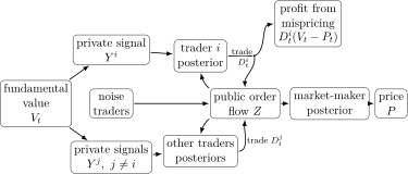
Figure 4.1. Information feedback around public order flow. The trader trades on its posterior. The same trade is a payoff action, earning $D_{t}^{i} (V_{t} - P_{t})$ , and a signal, because it enters public order flow. Other strategic trades and noise-trader demand also enter $Z$ . The market maker updates its posterior on public order flow and sets the price from it; the traders update on the same flow.

The belief-price method of Chapter 1 prices that second, intertemporal channel: here the beliefs a deviation manipulates are the ones the market maker and the other traders form from public order flow rather than from an abstract state signal. In Foster–Viswanathan a trader who has deviated carries one extra scalar, the gap between the equilibrium-path price and the realized price, to summarize past off-equilibrium play; here the deviation is priced at the margin. Perturb trader $i$ ’s order at time $t$ by a marginal spike $z$ . Because the order enters the public flow $Z$ , it changes every other observer’s signal history and so their noise-state estimates, in two parts: a shift in the old-history coordinates ( $r < t$ ) and a fresh coordinate born at the current date (the birth term). A deterministic forward-response map carries the seed through the observers’ filters, the other traders’ policy kernels, and the pricing rule. Its output is the future price response $p_{i} (τ, t; z)$ . The adjoint system, the discounted dual of this map, prices the seed by integrating, with discount rate $ρ$ , $(D_{τ}^{i})^{⊤} p_{i} (τ, t; z)$ , the future execution cost the price response creates.

4.2The stationary Kyle–Back market

Dictionary from Chapter 1.

The market notation below specializes the baseline calculus. The physical state $X$ contains the fundamental, price, and mispricing coordinates, while $D^{i}$ is trader $i$ ’s order rate. The market maker is observer $0$ , and the belief price $H^{k, i}$ prices movements of observer $k$ ’s posterior. The only persistent new market object is the price-impact map $Λ$ , the instantaneous map from an order innovation to a price innovation.

Spike terminology.

A spike is the marginal order deviation. Its seed is the immediate state and filter displacement created at the spike time, and its forward response carries that seed to later dates. Movements of coordinates already present before the spike are old-history effects.

Fix a discount rate $ρ > 0$ and a deviating trader $i$ . Viewed from a finite anchor time $t$ , all past shocks $r < t$ enter the state only through the observers’ filter kernels $F_{t}^{j} (r, u), r, u < t, j \in {0, 1, \dots, n} .$ Here $0$ is the market maker and $1, \dots, n$ are traders. For a deviation by trader $i$ , the shifted observer blocks are $O_{i} := {0} \cup {j : 1 \leq j \leq n, j \neq = i} .$

4.2.1Primitive shocks and covariance selectors

One standard $d$ -dimensional two-sided Brownian noise $W$ generates all randomness. Economic shocks are fixed linear combinations of the increments $d W$ : $d V_{t} d Z_{t} d Y_{t}^{j} = Σ_{V}^{1/2} E^{V} d W_{t}, = j = 1 \sum n D_{t}^{j} d t + Σ_{Z}^{1/2} E^{Z} d W_{t}, = B_{X}^{Y, j} (V_{t} - P_{t}) d t + Σ_{Y, j}^{1/2} E^{j} d W_{t}, j = 1, \dots, n . (4.2.2)$ Here $V_{t} \in R^{q}$ and $Z_{t} \in R^{q}$ are levels relative to an arbitrary finite origin; changing the origin adds a common formal level that cancels from $M_{t}^{i}$ (Section 4.2.3). The market maker prices competitively and each trader values the asset from its own filtration, $P_{t} = E [V_{t} ∣ F_{t}^{0}], V_{t}^{i} = E [V_{t} ∣ F_{t}^{i}], (4.2.3)$ relative to the same origin. The first equality is imposed as a consistency rule. The matrices $E^{V}, E^{Z}, E^{j}$ are selector maps into primitive-shock channels. Throughout this chapter their rows are normalized, $E^{V} (E^{V})^{⊤} = I, E^{Z} (E^{Z})^{⊤} = I, E^{j} (E^{j})^{⊤} = I,$ with identities of the appropriate dimensions. The matrices $Σ_{V}^{1/2}$ , $Σ_{Z}^{1/2}$ , and $Σ_{Y, j}^{1/2}$ therefore carry the covariance scale, so $Cov (d V_{t}) = Σ_{V} d t, Cov (Σ_{Z}^{1/2} E^{Z} d W_{t}) = Σ_{Z} d t, Cov (Σ_{Y, j}^{1/2} E^{j} d W_{t}) = Σ_{Y, j} d t .$ Cross-covariances enter through $Σ_{Y}^{jk} := Σ_{Y, j}^{1/2} E^{j} (E^{k})^{⊤} Σ_{Y, k}^{1/2} .$

The lack of correlation between fundamental factors and noise-trader factors is the orthogonality condition $E^{V} (E^{Z})^{⊤} = 0.$ In the baseline version the private-signal noise blocks are also orthogonal to the fundamental and noise-trader blocks: $E^{V} (E^{j})^{⊤} = 0, E^{Z} (E^{j})^{⊤} = 0, j = 1, \dots, n .$ A raw order-flow spike therefore has no direct private-signal noise component; any effect on $Y^{j}$ comes through the drift $B_{X}^{Y, j} (V_{t} - P_{t})$ .

4.2.2Standing assumptions

Assumption 4.1 (Stationary admissible environment). The following conditions stand throughout the chapter.

The discount rate satisfies $ρ > 0$ .
The covariance $Σ_{Z}$ is inverted only on the traded order-flow support. If $Σ_{Z}$ is singular, $Σ_{Z}^{- 1/2}$ denotes the corresponding pseudoinverse square-root map.
Policy kernels are predictable and have zero diagonal trace: $D_{t}^{j} (t) = 0$ .
The notation distinguishes noise-state and primitive coordinates. The kernel $D_{t}^{j} (u)$ multiplies trader $j$ ’s noise-state increment, while $D_{t}^{j}$ and $D_{W, t}^{j} (u)$ denote raw demand and its primitive-shock response kernel.
The stationary kernels are square-integrable enough for the displayed stochastic integrals, convolutions, and conditional expectations.
The discounted belief prices satisfy the transversality condition in Definition 4.5 (Section 4.5).
If $Λ (t)$ of (4.3.17) is singular, read all first-order conditions as range equations. The pseudoinverse selects a representative only on the instantaneous impacted subspace.

4.2.3Discounted objective and finite mispricing

Write $D_{t}^{i}$ for trader $i$ ’s realized raw-demand control. Trader $i$ evaluates future profit from time $t$ by $J_{t}^{i} (D^{i}; D^{- i}) := E [\int_{t}^{\infty} e^{- ρ (τ - t)} (D_{τ}^{i})^{⊤} (V_{τ}^{i} - P_{τ}) d τ F_{t}^{i}] . (4.2.9)$ Only the mispricing $M_{t}^{i} := V_{t}^{i} - P_{t}$ will enter the first-order condition. At zero trading cost the best response is not unique. The computations of Section 4.8 therefore add a quadratic trading cost, which selects one best response and leaves the reported quantities converging as the cost vanishes.

Before expanding the filter response, write $p_{i} (τ, t; z)$ for the price movement at future time $τ$ caused by a raw spike $z \in R^{q}$ submitted by trader $i$ at time $t$ . By submitting a spike of length $h$ in direction $z$ , trader $i$ earns $z^{⊤} M_{t}^{i}$ now, to first order. The spike also changes the prices at which trader $i$ executes later, and the first variation of the continuation payoff is $z^{⊤} M_{t}^{i} - E [\int_{t}^{\infty} e^{- ρ (τ - t)} (D_{τ}^{i})^{⊤} p_{i} (τ, t; z) d τ F_{t}^{i}] . (4.2.11)$ At a best response this expression is zero for every $F_{t}^{i}$ -measurable spike direction $z$ , so the unexpanded spike stationarity condition is $z^{⊤} M_{t}^{i} = E [\int_{t}^{\infty} e^{- ρ (τ - t)} (D_{τ}^{i})^{⊤} p_{i} (τ, t; z) d τ F_{t}^{i}], z \in R^{q} . (4.2.12)$

Lemma 4.2 (Finite mispricing under an infinite past). Introduce a finite lower cutoff $a < t$ and set $V_{t}^{(a)} := \int_{a}^{t} Σ_{V}^{1/2} E^{V} d W_{s} .$ Let $V_{t}^{i, (a)}$ and $P_{t}^{(a)}$ be the corresponding trader- $i$ estimate and market-maker price. If the difference between the trader and market-maker filter kernels is square integrable on $(- \infty, t)$ , then $M_{t}^{i} = a ↓ - \infty lim (V_{t}^{i, (a)} - P_{t}^{(a)})$ exists in $L^{2}$ . The individual levels $V_{t}^{i, (a)}$ and $P_{t}^{(a)}$ may fail to converge as $a ↓ - \infty$ .

Proof. For each cutoff, both $V_{t}^{i, (a)}$ and $P_{t}^{(a)}$ are linear functionals of the primitive shock on $(a, t)$ . Their difference is the same primitive shock integrated against the difference of the two deterministic filter kernels. The stated square-integrability condition makes this family Cauchy in $L^{2}$ by Itô isometry. ◻

4.3The life of a trader’s order

A marginal order does three things at the instant it arrives. It re-weights everything the observers already believed, moving the old coordinates of their noise-states; it creates a new coordinate born at the current date; and it moves the price through the market maker’s filter.

4.3.1Order-flow block and filter kernels

The market maker observes order flow in normalized units, using $Σ_{Z}^{- 1/2} Z$ . Trader $j \geq 1$ observes this same order-flow channel plus its private signal. The selector $χ^{0} := I_{q}, χ^{j} := (I_{q} 0_{p_{j} - q, q}), j \geq 1,$ embeds a normalized order-flow increment into the $Z$ -block of trader $j$ ’s stacked observation, of dimension $p_{j}$ , and adds zero to the private-signal block.

For any trader $j$ , the same realized raw-demand process has two impulse-response representations, following the convention of Chapter 1: $D_{t}^{j} = \overset{ˉ}{D}_{t}^{j} + \int_{- \infty}^{t} D_{t}^{j} (u) d W_{t}^{j} (u) = \overset{ˉ}{D}_{t}^{j} + \int_{- \infty}^{t} D_{W, t}^{j} (u) d W_{u} . (4.3.2)$ The first integral writes the policy in trader $j$ ’s noise-state coordinates, $W_{t}^{j} (u) = E [W_{u} ∣ F_{t}^{j}]$ , the second the same raw demand in primitive-shock coordinates. The total primitive-coordinate order-flow drift is $D_{W, t}^{tot} (u) := j = 1 \sum n D_{W, t}^{j} (u), u < t .$ For each trader $j$ , the normalized drift of the private price signal is $Σ_{Y, j}^{- 1/2} B_{X}^{Y, j} (V_{t} - P_{t})$ . The price, a linear functional of the order-flow history the trader sees, is in $F_{t}^{j}$ , so it drops out of the innovation on and off the path, and only the fundamental’s kernel enters; write $Σ_{Y, j}^{- 1/2} B_{X}^{Y, j} V_{t} = \overline{C}_{t}^{Y, j} + \int_{- \infty}^{t} C_{t}^{Y, j} (u) d W_{u}, j = 1, \dots, n . (4.3.4)$ Its unresolved part is the bottom block of (4.3.11). The observation-drift kernels are $C_{t}^{0} (u) = Σ_{Z}^{- 1/2} D_{W, t}^{tot} (u),$ for the market maker, and $C_{t}^{j} (u) = (Σ_{Z}^{- 1/2} D_{W, t}^{tot} (u) C_{t}^{Y, j} (u)), j \geq 1,$ for trader $j$ .

The filter equations use the primitive objects each observer has not yet resolved. Let $Π^{0} := E^{Z, ⊤} E^{Z}, Π^{j} := E^{Z, ⊤} E^{Z} + E^{j, ⊤} E^{j}, j \geq 1.$ Each $Π^{k}$ collects the channels observer $k$ resolves at once: order flow for everyone, plus its own signal for a trader. The unresolved aggregate order-flow drift for observer $k \in {0, 1, \dots, n}$ is $D_{W, t}^{tot, k} (u) := D_{W, t}^{tot} (u) (I - Π^{k}) - \int_{- \infty}^{t} D_{W, t}^{tot} (r) F_{t}^{k} (r, u) d r . (4.3.8)$ The unresolved value kernel is $V_{t}^{k} (u) := Σ_{V}^{1/2} E^{V} (I - Π^{k}) - \int_{- \infty}^{t} Σ_{V}^{1/2} E^{V} F_{t}^{k} (r, u) d r . (4.3.9)$ Under the maintained orthogonality between fundamental shocks and contemporaneous observation-noise blocks, the first term in (4.3.9) is $Σ_{V}^{1/2} E^{V}$ .

The unresolved observation-drift kernels are then $C_{t}^{0} (u) = Σ_{Z}^{- 1/2} D_{W, t}^{tot, 0} (u), (4.3.10)$ and, for trader $j \geq 1$ , $C_{t}^{j} (u) = (Σ_{Z}^{- 1/2} D_{W, t}^{tot, j} (u) Σ_{Y, j}^{- 1/2} B_{X}^{Y, j} V_{t}^{j} (u)) . (4.3.11)$ The top block is the order-flow channel, the bottom the private price signal.

The compact old-history filter equation is $\partial_{t} F_{t}^{k} (r, u) = C_{t}^{k} (r)^{⊤} C_{t}^{k} (u), k = 0, 1, \dots, n, r, u < t . (4.3.12)$ The market-maker filter evolves by $\partial_{t} F_{t}^{0} (r, u) = D_{W, t}^{tot, 0} (r)^{⊤} Σ_{Z}^{- 1} D_{W, t}^{tot, 0} (u), r, u < t, (4.3.13)$ with birth traces, the kernel’s boundary values at the coordinate born at $t$ , $F_{t}^{0} (r, t) = D_{W, t}^{tot, 0} (r)^{⊤} Σ_{Z}^{- 1/2} E^{Z}, F_{t}^{0} (t, u) = E^{Z, ⊤} Σ_{Z}^{- 1/2} D_{W, t}^{tot, 0} (u) . (4.3.14)$ For trader $j \geq 1$ , the old-history equation is $\partial_{t} F_{t}^{j} (r, u) = D_{W, t}^{tot, j} (r)^{⊤} Σ_{Z}^{- 1} D_{W, t}^{tot, j} (u) + V_{t}^{j} (r)^{⊤} (B_{X}^{Y, j})^{⊤} Σ_{Y, j}^{- 1} B_{X}^{Y, j} V_{t}^{j} (u), r, u < t . (4.3.15)$ Its birth traces are $F_{t}^{j} (r, t) = F_{t}^{j} (t, u) = D_{W, t}^{tot, j} (r)^{⊤} Σ_{Z}^{- 1/2} E^{Z} + V_{t}^{j} (r)^{⊤} (B_{X}^{Y, j})^{⊤} Σ_{Y, j}^{- 1/2} E^{j}, E^{Z, ⊤} Σ_{Z}^{- 1/2} D_{W, t}^{tot, j} (u) + E^{j, ⊤} Σ_{Y, j}^{- 1/2} B_{X}^{Y, j} V_{t}^{j} (u) . (4.3.16)$

4.3.2From an order to a price move

Figure 4.2. Order-flow news first becomes a normalized order-flow innovation, then a market-maker noise-state movement, and then a price movement.

The price-impact map is $Λ (t) := (\int_{- \infty}^{t} Σ_{V}^{1/2} E^{V} C_{t}^{0} (r)^{⊤} d r) Σ_{Z}^{- 1/2} . (4.3.17)$ An order moves the price only by moving the market maker’s innovations (Figure 4.2). By the factor orthogonality $E^{V} E^{Z, ⊤} = 0$ , the birth term of the transpose contraction $B^{0⊤}$ , (1.4.9) of Chapter 1, vanishes, and $Λ (t) = Σ_{V}^{1/2} E^{V} B^{0⊤} Σ_{Z}^{- 1/2}$ . A raw order-flow spike in a direction $z \in Ker Λ (t)$ , equivalently with $\int_{- \infty}^{t} C_{t}^{0} (r)^{⊤} Σ_{Z}^{- 1/2} z d r \in Ker (Σ_{V}^{1/2} E^{V})$ , produces no instantaneous market-maker price response; its price effects are future ones, carried by the forward response and belief-price terms below.

A strategic unit spike by trader $i$ places the old-history seeds $φ_{i}^{0} (t, r) := C_{t}^{0} (r)^{⊤} Σ_{Z}^{- 1/2}, (4.3.18)$ and, for trader observers $j \neq = i$ , $φ_{i}^{j} (t, r) := C_{t}^{j} (r)^{⊤} χ^{j} Σ_{Z}^{- 1/2}, j = 1, \dots, n, j \neq = i .$ The same spike creates the birth seeds $ψ_{i}^{0} (t) := E^{Z, ⊤} Σ_{Z}^{- 1/2}, (4.3.20)$ and, for trader observers $j \neq = i$ , $ψ_{i}^{j} (t) := E^{Z, ⊤} Σ_{Z}^{- 1/2}, j = 1, \dots, n, j \neq = i . (4.3.21)$ The two birth seeds coincide because the spike enters trader $j$ ’s stacked observation only through the common order-flow block; its private-signal noise component is zero.

Remark 4.3 (Order-flow martingales and primitive drift). Back’s continuous-time equilibrium makes total order flow a martingale in the market-maker filtration. In the notation here this martingale property is imposed after conditioning on the market maker’s information. The kernel $C^{0}$ is the primitive-shock impulse response of the normalized order-flow drift, while $C^{0}$ is the part of that drift not yet resolved by the market-maker filter. The market-maker innovation can then be a martingale even though $C^{0}$ is nonzero. In the pure risk-neutral Kyle–Back benchmark, with no inventory or risk-premium motive for the market maker, the predictable component of public order flow is exactly the part subtracted by the filter. Section 4.8.1 works out the special case $C^{0} = C^{0}$ , in which no part of the primitive order-flow drift is already resolved by the market maker.

4.3.3Spike seed measure and immediate response

For a raw spike direction $z \in R^{q}$ submitted by trader $i$ , combine the old-history and birth parts into the seed measure on $(- \infty, t]$ $d η_{i}^{0} (t, u; z) d η_{i}^{j} (t, u; z) = φ_{i}^{0} (t, u) z d u + ψ_{i}^{0} (t) z δ_{t} (d u), = φ_{i}^{j} (t, u) z d u + ψ_{i}^{j} (t) z δ_{t} (d u), j = 1, \dots, n, j \neq = i . (4.3.22) (4.3.23)$

The other traders’ immediate change in demand.

The old-history part of a spike generates the immediate opponent demand response $δ D_{Σ, t}^{(- i)} (z) = R^{i} (t) z, R^{i} (t) = j = 1 j \neq = i \sum n \int_{- \infty}^{t} D_{t}^{j} (u) C_{t}^{j} (u)^{⊤} χ^{j} Σ_{Z}^{- 1/2} d u . (4.3.24)$ $R^{i} (t)$ leaves out the birth atom, because the policy kernel is predictable and has zero trace at $u = t$ , so no instantaneous term $D_{t}^{j} (t) ψ_{i}^{j} z$ appears.

4.4Forward response

Write $δ w_{τ}^{j} (r)$ for the perturbation of observer $j$ ’s noise-state coordinate $r$ at future time $τ$ , in density form: $d_{r} δ W_{τ}^{j} (r) = δ w_{τ}^{j} (r) d r$ . The change in the other traders’ total demand at time $τ$ is $δ D_{Σ, τ}^{(- i)} = j = 1 j \neq = i \sum n \int_{- \infty}^{τ} D_{τ}^{j} (u) δ w_{τ}^{j} (u) d u . (4.4.1)$ The old-history perturbations satisfy $\partial_{τ} δ w_{τ}^{0} (r) \partial_{τ} δ w_{τ}^{j} (r) = C_{τ}^{0} (r)^{⊤} [Σ_{Z}^{- 1/2} δ D_{Σ, τ}^{(- i)} - \int_{- \infty}^{τ} C_{τ}^{0} (u) δ w_{τ}^{0} (u) d u], = C_{τ}^{j} (r)^{⊤} [χ^{j} Σ_{Z}^{- 1/2} δ D_{Σ, τ}^{(- i)} - \int_{- \infty}^{τ} C_{τ}^{j} (u) δ w_{τ}^{j} (u) d u], (4.4.2) (4.4.3)$ for $r < τ$ and $j = 1, \dots, n$ , $j \neq = i$ . The coordinate born at the current date is $δ w_{τ}^{0} (τ) δ w_{τ}^{j} (τ) = E^{Z, ⊤} [Σ_{Z}^{- 1/2} δ D_{Σ, τ}^{(- i)} - \int_{- \infty}^{τ} C_{τ}^{0} (u) δ w_{τ}^{0} (u) d u], = (E^{Z, ⊤} E^{j, ⊤}) [χ^{j} Σ_{Z}^{- 1/2} δ D_{Σ, τ}^{(- i)} - \int_{- \infty}^{τ} C_{τ}^{j} (u) δ w_{τ}^{j} (u) d u], (4.4.4) (4.4.5)$ for $j = 1, \dots, n$ , $j \neq = i$ . Only the market maker’s noise-state is read directly into a price movement: $δ P_{τ} = \int_{- \infty}^{τ} Σ_{V}^{1/2} E^{V} δ w_{τ}^{0} (s) d s .$ This perturbation is finite by the argument of Lemma 4.2.

Linearity lets one propagate a generic initial perturbation of an observer’s noise-state and contract that response against the seed generated by a raw order-flow spike.

For $m, k \in O_{i}$ , define $G_{τ \leftarrow t}^{m \leftarrow k} (s \leftarrow u)$ as the distributional kernel that maps an initial perturbation in observer $k$ ’s noise-state coordinate $u \leq t$ at time $t$ into the perturbation of observer $m$ ’s coordinate $s \leq τ$ at time $τ$ : $(G_{τ \leftarrow t}^{m \leftarrow k} η) (s) := \int_{(- \infty, t]} G_{τ \leftarrow t}^{m \leftarrow k} (s \leftarrow u) d η (u), τ \geq t . (4.4.7)$ The initial condition is $G_{t \leftarrow t}^{m \leftarrow k} = 1_{{m = k}} Id$ . Equivalently, $G_{t \leftarrow t}^{m \leftarrow m} (s \leftarrow u) = δ (s - u)$ in the distributional sense. Read all identities involving the Dirac initial kernel $δ (s - u)$ weakly, after pairing with the finite seed measure above.

For $s < τ$ , the forward-response kernels satisfy the same old-history equations as the perturbations. For the market maker’s noise-state, $\partial_{τ} G_{τ \leftarrow t}^{0 \leftarrow k} (s \leftarrow u) = C_{τ}^{0} (s)^{⊤} [Σ_{Z}^{- 1/2} j = 1 j \neq = i \sum n \int_{- \infty}^{τ} D_{τ}^{j} (r) G_{τ \leftarrow t}^{j \leftarrow k} (r \leftarrow u) d r - \int_{- \infty}^{τ} C_{τ}^{0} (r) G_{τ \leftarrow t}^{0 \leftarrow k} (r \leftarrow u) d r] . (4.4.8)$ For the noise-state of a trader $m \neq = i$ , $\partial_{τ} G_{τ \leftarrow t}^{m \leftarrow k} (s \leftarrow u) = C_{τ}^{m} (s)^{⊤} [χ^{m} Σ_{Z}^{- 1/2} j = 1 j \neq = i \sum n \int_{- \infty}^{τ} D_{τ}^{j} (r) G_{τ \leftarrow t}^{j \leftarrow k} (r \leftarrow u) d r - \int_{- \infty}^{τ} C_{τ}^{m} (r) G_{τ \leftarrow t}^{m \leftarrow k} (r \leftarrow u) d r] . (4.4.9)$ The coordinate born at $s = τ$ is $G_{τ \leftarrow t}^{0 \leftarrow k} (τ \leftarrow u) = E^{Z, ⊤} [Σ_{Z}^{- 1/2} j = 1 j \neq = i \sum n \int_{- \infty}^{τ} D_{τ}^{j} (r) G_{τ \leftarrow t}^{j \leftarrow k} (r \leftarrow u) d r - \int_{- \infty}^{τ} C_{τ}^{0} (r) G_{τ \leftarrow t}^{0 \leftarrow k} (r \leftarrow u) d r], (4.4.10)$ for the market maker. For the noise-state of a trader $m \neq = i$ , split the stacked residual into its common order-flow and private-signal components: $E_{Z, τ \leftarrow t}^{m \leftarrow k} (u) E_{Y, τ \leftarrow t}^{m \leftarrow k} (u) := Σ_{Z}^{- 1/2} j = 1 j \neq = i \sum n \int_{- \infty}^{τ} D_{τ}^{j} (r) G_{τ \leftarrow t}^{j \leftarrow k} (r \leftarrow u) d r - \int_{- \infty}^{τ} C_{τ}^{0} (r) G_{τ \leftarrow t}^{m \leftarrow k} (r \leftarrow u) d r, := - \int_{- \infty}^{τ} C_{τ}^{Y, m} (r) G_{τ \leftarrow t}^{m \leftarrow k} (r \leftarrow u) d r . (4.4.11) (4.4.12)$ Then the born coordinate is $G_{τ \leftarrow t}^{m \leftarrow k} (τ \leftarrow u) = E^{Z, ⊤} E_{Z, τ \leftarrow t}^{m \leftarrow k} (u) + E^{m, ⊤} E_{Y, τ \leftarrow t}^{m \leftarrow k} (u), m \neq = i . (4.4.13)$

The future price movement at $τ$ caused by the raw spike is the sum of the price responses generated by each observer whose beliefs the spike moves: $p_{i} (τ, t; z) := k \in O_{i} \sum \int_{(- \infty, t]} p^{k} (τ, t, u) d η_{i}^{k} (t, u; z) . (4.4.14)$ The channel price-response density is $p^{k} (τ, t, u) := \int_{- \infty}^{τ} Σ_{V}^{1/2} E^{V} G_{τ \leftarrow t}^{0 \leftarrow k} (s \leftarrow u) d s, k \in O_{i} . (4.4.15)$

Proposition 4.4 (Instantaneous price impact). For every raw spike direction $z$ , $p_{i} (t, t; z) = Λ (t) z . (4.4.16)$

Proof. At $τ = t$ the forward response is the identity on the seed’s own block and zero elsewhere, so only the market maker’s seed reaches the price: $G_{t \leftarrow t}^{0 \leftarrow 0} (s \leftarrow u) = δ (s - u)$ . Contracting this with the old-history market-maker seed (4.3.18) gives $Λ (t) z$ . The birth atom in the market-maker block would contribute $Σ_{V}^{1/2} E^{V} E^{Z, ⊤} Σ_{Z}^{- 1/2} z$ , zero by the fundamental/order-flow orthogonality condition. ◻

4.5Discounted belief prices and mispricing drift

Definition 4.5 (Discounted belief prices). For the market maker and for each trader observer $j \neq = i$ , define $H^{j, i}$ by $\int_{t}^{\infty} e^{- ρ (τ - t)} (D_{τ}^{i})^{⊤} δ P_{τ} d τ = \int_{- \infty}^{t} H_{t}^{0, i} (r) η^{0} (r) d r + j = 1 j \neq = i \sum n \int_{- \infty}^{t} H_{t}^{j, i} (r) η^{j} (r) d r, (4.5.1)$ where $δ P_{τ}$ is the price response when $δ w$ solves the forward perturbation equations with initial perturbation $η$ at time $t$ . The belief price $H_{t}^{j, i} (r)$ is the marginal discounted future execution cost to trader $i$ of shifting observer $j$ ’s noise-state at $r$ . The infinite-horizon replacement for the finite terminal condition is the transversality condition $τ \to \infty lim e^{- ρ (τ - t)} \int_{- \infty}^{τ} H_{τ}^{0, i} (r) δ w_{τ}^{0} (r) d r + j = 1 j \neq = i \sum n \int_{- \infty}^{τ} H_{τ}^{j, i} (r) δ w_{τ}^{j} (r) d r = 0$ for admissible perturbations.

Substituting the total price response, channel by channel, into the discounted future execution cost isolates the recurring bracket $H_{t}^{k, i} (u) = \int_{t}^{\infty} e^{- ρ (τ - t)} (D_{τ}^{i})^{⊤} p^{k} (τ, t, u) d τ, k \in O_{i} . (4.5.3)$ Equation (4.5.3) has the same row/column convention as Definition 4.5; the endpoint value $H_{t}^{k, i} (t)$ is the discounted value of the born coordinate.

Contracting $H_{t}^{k, i}$ against the unresolved drift kernel $C_{t}^{k}$ on old history and against the birth selector at $u = t$ gives the stationary form of the transpose contraction (1.4.9) of Chapter 1. For the market maker, $H_{t}^{0, i} B^{0⊤} := \int_{- \infty}^{t} H_{t}^{0, i} (s) C_{t}^{0} (s)^{⊤} d s + H_{t}^{0, i} (t) E^{Z, ⊤} . (4.5.4)$ For a trader observer $j \neq = i$ , $H_{t}^{j, i} B^{j ⊤} := \int_{- \infty}^{t} H_{t}^{j, i} (s) C_{t}^{j} (s)^{⊤} d s + H_{t}^{j, i} (t) (E^{Z, ⊤} E^{j, ⊤}) . (4.5.5)$ The market maker observes only order flow, so its row is a pure $Z$ block. For trader observers, split $H_{t}^{j, i} B^{j ⊤} = ((H_{t}^{j, i} B^{j ⊤})_{Z}, (H_{t}^{j, i} B^{j ⊤})_{Y})$ into order-flow and private-signal blocks. The value of one normalized aggregate order-flow innovation is $β_{t}^{i} := H_{t}^{0, i} B^{0⊤} + j = 1 j \neq = i \sum n (H_{t}^{j, i} B^{j ⊤})_{Z} . (4.5.6)$

Theorem 4.6 (Discounted backward system for the belief prices). Under the transversality condition in Definition 4.5, the market maker’s belief price solves $(ρ - \partial_{t}) H_{t}^{0, i} (r) = price move (D_{t}^{i})^{⊤} Σ_{V}^{1/2} E^{V} - Z self-correction H_{t}^{0, i} B^{0⊤} Σ_{Z}^{- 1/2} D_{W, t}^{tot} (r) . (4.5.7)$ For every trader observer $j = 1, \dots, n$ , $j \neq = i$ , $(ρ - \partial_{t}) H_{t}^{j, i} (r) = active demand β_{t}^{i} Σ_{Z}^{- 1/2} D_{t}^{j} (r) - Z self-correction (H_{t}^{j, i} B^{j ⊤})_{Z} Σ_{Z}^{- 1/2} D_{W, t}^{tot} (r) - Y self-correction (H_{t}^{j, i} B^{j ⊤})_{Y} C^{Y, j} (t, r) . (4.5.8)$ There is no equation for $H^{i, i}$ , because trader $i$ knows its own order, so the order does not move trader $i$ ’s beliefs.

No $C^{0}$ appears in the market-maker source, because the seed (4.3.18) already carries it. An opponent’s order does not move the price directly; it enters the common $Z$ observation, the market maker and the other traders update on it, and the market maker’s update moves the price.

Remark 4.7 (The filter subtracts $C$ , not another $C$ ). The forward filter term has the form $C^{j ⊤} [\dots - \int C^{j} δ w^{j}] .$ $H^{j, i} B^{j ⊤}$ already absorbs the factor $C^{j}$ . The remaining kernel is the observation drift $C^{j}$ , which is why the self-correction terms in Theorem 4.6 contain $Σ_{Z}^{- 1/2} D_{W}^{tot}$ and $C^{Y, j}$ .

A marginal spike inserts the old-history seeds $φ_{i}^{j}$ and the birth seeds $ψ_{i}^{j}$ into the observer blocks, so the first-order condition is $(M_{t}^{i})^{⊤} = E [\int_{- \infty}^{t} H_{t}^{0, i} (r) φ_{i}^{0} (t, r) d r + H_{t}^{0, i} (t) ψ_{i}^{0} (t) + j = 1 j \neq = i \sum n (\int_{- \infty}^{t} H_{t}^{j, i} (r) φ_{i}^{j} (t, r) d r + H_{t}^{j, i} (t) ψ_{i}^{j} (t)) F_{t}^{i}] . (4.5.9)$

Differentiating the stationary kernel representation and using (4.3.12), $d M_{t}^{i} = {\int_{- \infty}^{t} Σ_{V}^{1/2} E^{V} \int_{- \infty}^{t} (C_{t}^{i} (u)^{⊤} C_{t}^{i} (s) - C_{t}^{0} (u)^{⊤} C_{t}^{0} (s)) d u d W_{s}} d t + d M_{t} .$ The martingale $M$ collects the increment at the boundary $s = t$ . The other boundary term of the inner integral, at $u = t$ , would pair the contemporaneous observation noise with $Σ_{V}^{1/2} E^{V}$ ; it vanishes because the selectors are orthogonal, $E^{V} E^{Z ⊤} = E^{V} E^{i ⊤} = 0$ . The term in which $C^{i}$ multiplies trader $i$ ’s own innovation vanishes after conditioning on $F_{t}^{i}$ , because $C^{i}$ is the innovation gain of trader $i$ ’s own filter, so its old-history component is orthogonal to trader $i$ ’s information at time $t$ . Hence $drift_{F_{t}^{i}} (M^{i}) = - \int_{- \infty}^{t} K_{t}^{0} (s) d W_{t}^{i} (s), K_{t}^{0} (s) := Σ_{V}^{1/2} E^{V} \int_{- \infty}^{t} C_{t}^{0} (u)^{⊤} C_{t}^{0} (s) d u . (4.5.11)$

Lemma 4.8 (The predictable drift lies in the price-impact range). For every old-history coordinate $s < t$ , $K_{t}^{0} (s) = Λ (t) Σ_{Z}^{1/2} C_{t}^{0} (s) . (4.5.12)$ Consequently the predictable drift in (4.5.11) lies in $Range (Λ (t))$ , with raw-demand preimage $Σ_{Z}^{1/2} C_{t}^{0} (s)$ .

Proof. Substitute the definition of $Λ (t)$ in (4.3.17) and use $Σ_{Z}^{- 1/2} Σ_{Z}^{1/2}$ as the identity on the traded order-flow support. ◻

Proof of Theorem 4.6. Let $δ D_{t} := j = 1 j \neq = i \sum n \int_{- \infty}^{t} D_{t}^{j} (u) δ w_{t}^{j} (u) d u,$ and $P_{t} (H, δ w) := \int_{- \infty}^{t} H_{t}^{0, i} (r) δ w_{t}^{0} (r) d r + j = 1 j \neq = i \sum n \int_{- \infty}^{t} H_{t}^{j, i} (r) δ w_{t}^{j} (r) d r .$ On old history coordinates $r < t$ , differentiating $P_{t}$ gives the interior terms and the contribution of the coordinates born at the current date $H_{t}^{0, i} (t) δ w_{t}^{0} (t) + j = 1 j \neq = i \sum n H_{t}^{j, i} (t) δ w_{t}^{j} (t) .$ After substituting the old-coordinate equations (4.4.2)–(4.4.3) and the birth conditions (4.4.4)–(4.4.5), the value assigned to an observation residual is the full contraction (4.5.4)–(4.5.5). The active-demand part contributes $H_{t}^{0, i} B^{0⊤} Σ_{Z}^{- 1/2} δ D_{t} + j = 1 j \neq = i \sum n (H_{t}^{j, i} B^{j ⊤})_{Z} Σ_{Z}^{- 1/2} δ D_{t} = β_{t}^{i} Σ_{Z}^{- 1/2} δ D_{t},$ and the self-correction part contributes $- H_{t}^{0, i} B^{0⊤} \int_{- \infty}^{t} Σ_{Z}^{- 1/2} D_{W, t}^{tot} (u) δ w_{t}^{0} (u) d u - j = 1 j \neq = i \sum n [(H_{t}^{j, i} B^{j ⊤})_{Z} \int_{- \infty}^{t} Σ_{Z}^{- 1/2} D_{W, t}^{tot} (u) δ w_{t}^{j} (u) d u + (H_{t}^{j, i} B^{j ⊤})_{Y} \int_{- \infty}^{t} C_{t}^{Y, j} (u) δ w_{t}^{j} (u) d u] .$ Equations (4.5.7)–(4.5.8) cancel these terms. The remaining terms are $\frac{d}{d t} P_{t} (H, δ w) = ρ P_{t} (H, δ w) - (D_{t}^{i})^{⊤} \int_{- \infty}^{t} Σ_{V}^{1/2} E^{V} δ w_{t}^{0} (r) d r = ρ P_{t} (H, δ w) - (D_{t}^{i})^{⊤} δ P_{t} .$ Equivalently, $\frac{d}{d t} (e^{- ρ (t - s)} P_{t} (H, δ w)) = - e^{- ρ (t - s)} (D_{t}^{i})^{⊤} δ P_{t}$ for any fixed anchor $s$ . Integrating from $s$ to $\infty$ and using transversality gives (4.5.1). Since (4.5.1) determines $H$ uniquely as a functional on seeds, this solution is the belief price. ◻

4.6Moving the spike date

Dictionary from Chapter 3.

The analysis runs in that chapter’s stationary lag coordinates, and one convention differs. Chapter 3 splits each stationary object into a deterministic mean and a deterministic kernel against past shocks, as in (3.2.4); here the random object is kept with its calendar subscript. So $h_{t}^{k, i} (b)$ of (4.6.3) is that chapter’s random belief price $H_{t}^{k, i} (b)$ in age coordinates, not its deterministic kernel $h^{k, i} (b, ℓ)$ . The unresolved innovation kernels $c^{0}, c^{j}$ are its $\tilde{c}^{k, Z}, \tilde{c}^{k, Y}$ , and the total-policy kernel $D_{W, t}^{tot} (u)$ is the sum over traders of its control kernels $d_{W}^{m}$ at age $b = t - u$ .

The raw-spike condition (4.2.12) holds at every spike date, and moving the spike date moves the seed it creates. Proposition 4.9 records the result; paired with the mispricing drift (4.5.11), it gives the first-order condition of Section 4.7.

Write the raw-spike FOC (4.2.12) as a pairing of belief prices with the seed: $z^{⊤} M_{t}^{i} = E [S_{t}^{i} (z) F_{t}^{i}], (4.6.1)$ Here $h_{t}^{k, i} (b)$ is the belief price of observer $k$ at shock age $b$ , and $ϕ_{i}^{k} (b)$ and $ψ_{i}^{k}$ are the old-history and birth seeds trader $i$ ’s spike leaves in observer $k$ ’s filter, all three in the stationary lag coordinates set out in (4.6.3)–(4.6.4) below. In those coordinates, $S_{t}^{i} (z) := k \in O_{i} \sum (\int_{0}^{\infty} h_{t}^{k, i} (b) ϕ_{i}^{k} (b) z d b + h_{t}^{k, i} (0) ψ_{i}^{k} z) . (4.6.2)$

To differentiate this identity in the spike date, use stationary lag coordinates. In a stationary solution, the old-history derivative of the seed is a derivative in the age of the shock. Set $b = t - u$ , the coordinate age of the lag convention (3.1.5) of Chapter 3, and write $H_{t}^{k, i} (t - b) = h_{t}^{k, i} (b), φ_{i}^{k} (t, t - b) = ϕ_{i}^{k} (b), k \in O_{i} . (4.6.3)$ The old-history seed densities and birth matrices are $ϕ_{i}^{0} (b) = c^{0} (b)^{⊤} Σ_{Z}^{- 1/2}, ϕ_{i}^{j} (b) = c^{j} (b)^{⊤} χ^{j} Σ_{Z}^{- 1/2}, ψ_{i}^{0} = ψ_{i}^{j} = E^{Z, ⊤} Σ_{Z}^{- 1/2} . (4.6.4)$ For old-history coefficients, $C_{t}^{0} (t - b) = c^{0} (b), C_{t}^{j} (t - b) = c^{j} (b), C_{t}^{k} (t - b) = c^{k} (b), (4.6.5)$ where $c^{0} (b) = Σ_{Z}^{- 1/2} d_{W}^{tot} (b), c^{j} (b) = (Σ_{Z}^{- 1/2} d_{W}^{tot} (b) c^{Y, j} (b)), j \neq = i . (4.6.6)$ Here $d_{W}^{tot} (b) = D_{W, t}^{tot} (t - b)$ , $d^{j} (b) = D_{t}^{j} (t - b)$ , and $c^{Y, j} (b) = C_{t}^{Y, j} (t - b)$ . Each identity below holds as an $F_{t}^{i}$ -conditional expectation; read it as holding for the mean and for every coefficient of $d W_{t}^{i} (s)$ in the representation (4.7.3). In lag coordinates the adjoint equations of Theorem 4.6 read $(ρ - \partial_{t}) H_{t}^{k, i} (t - b) = s_{t}^{k, i} (b)$ , with source terms $s_{t}^{0, i} (b) := (D_{t}^{i})^{⊤} Σ_{V}^{1/2} E^{V} - H_{t}^{0, i} B^{0⊤} c^{0} (b), (4.6.7)$ for the market-maker block, and $s_{t}^{j, i} (b) := β_{t}^{i} Σ_{Z}^{- 1/2} d^{j} (b) - H_{t}^{j, i} B^{j ⊤} c^{j} (b), j \neq = i, (4.6.8)$ the second term of each being the value of the drift the observer’s filter already predicted, in the stacked form (4.6.6).

Moving the spike date also moves the seed. Its density transports in age, its support gains the point $b = 0$ , and the birth atom ages. At a fixed belief price the three contribute $k \in O_{i} \sum (\int_{0}^{\infty} h_{t}^{k, i} (b) \partial_{b} ϕ_{i}^{k} (b) z d b + h_{t}^{k, i} (0) ϕ_{i}^{k} (0) z - \partial_{b} h_{t}^{k, i} (0) ψ_{i}^{k} z) . (4.6.9)$

Proposition 4.9 (Drift of the spike condition as the spike date moves). For every raw direction $z$ , $drift E [S_{t}^{i} (z) F_{t}^{i}] = ρ z^{⊤} M_{t}^{i} - z^{⊤} Λ (t)^{⊤} D_{t}^{i} + z^{⊤} V_{t}^{i}, (4.6.10)$ where the wedge, the market form of the information wedge $v^{i}$ of (3.2.6), is $z^{⊤} V_{t}^{i} = E [k \in O_{i} \sum H_{t}^{k, i} B^{k ⊤} \int_{0}^{\infty} c^{k} (b) ϕ_{i}^{k} (b) z d b - β_{t}^{i} Σ_{Z}^{- 1/2} R^{i} (t) z + k \in O_{i} \sum (\int_{0}^{\infty} h_{t}^{k, i} (b) \partial_{b} ϕ_{i}^{k} (b) z d b + h_{t}^{k, i} (0) ϕ_{i}^{k} (0) z - \partial_{b} h_{t}^{k, i} (0) ψ_{i}^{k} z) F_{t}^{i}] . (4.6.11)$ The first line is the value of the drift each observer’s filter already predicted and subtracts from the seed, minus the value of the immediate opponent response; the second is the seed’s own motion (4.6.9).

Proof. $S_{t}^{i} (z) = ⟨ H_{t}, η_{t} ⟩$ pairs the belief prices with the seed measure (4.3.22)–(4.3.23), and both factors move with $t$ . Pathwise, Theorem 4.6 gives $\partial_{t} H_{t}^{k, i} (u) = ρ H_{t}^{k, i} (u) - s_{t}^{k, i} (u)$ at every fixed coordinate $u \leq t$ ; paired with the seed this is $ρ S_{t}^{i} (z) - ⟨ s, η_{t} ⟩$ . By (4.6.7)–(4.6.8), (4.3.17) and (4.3.24), $⟨ s, η_{t} ⟩ = z^{⊤} Λ (t)^{⊤} D_{t}^{i} + β_{t}^{i} Σ_{Z}^{- 1/2} R^{i} (t) z - k \in O_{i} \sum H_{t}^{k, i} B^{k ⊤} \int_{0}^{\infty} c^{k} (b) ϕ_{i}^{k} (b) z d b,$ the atom contributing nothing, since $E^{V} E^{Z, ⊤} = 0$ and the policy kernels have zero trace at age $0$ . The seed’s motion at a fixed belief price is (4.6.9), with $\partial_{u} H_{t}^{k, i} (u) ∣_{u = t} = - \partial_{b} h_{t}^{k, i} (0)$ . Summing, $d S_{t}^{i} (z) / d t = ρ S_{t}^{i} (z) - ⟨ s, η_{t} ⟩ + (4.6.9)$ pathwise. Conditioning, $E [S_{t + d t} ∣ F_{t + d t}^{i}] - E [S_{t} ∣ F_{t}^{i}] = E [S_{t + d t} - S_{t} ∣ F_{t + d t}^{i}] + (E [S_{t} ∣ F_{t + d t}^{i}] - E [S_{t} ∣ F_{t}^{i}])$ , and the second bracket is an $F^{i}$ -martingale increment, so the $F_{t}^{i}$ -drift of $E [S_{t}^{i} (z) ∣ F_{t}^{i}]$ is the conditional expectation of the pathwise derivative. Finally $E [S_{t}^{i} (z) ∣ F_{t}^{i}] = z^{⊤} M_{t}^{i}$ by (4.6.1), which turns $ρS$ into $ρ z^{⊤} M_{t}^{i}$ . ◻

4.7Stationary best response and equilibrium

A trader’s order, priced at impact, splits into a trade on the information gap, an impatience term, and the wedge. The information gap is the trader’s estimate of the unresolved total order flow.

Theorem 4.10 (Stationary best response to a stationary profile). Fix a stationary candidate profile of the other traders’ primitive-coordinate policy kernels and associated filter kernels. Under Assumption 4.1, trader $i$ ’s best response satisfies the level condition (4.5.9) and its $F_{t}^{i}$ -drift form $Λ (t)^{⊤} D_{t}^{i} - Λ (t) \int_{- \infty}^{t} Σ_{Z}^{1/2} C_{t}^{0} (s) d W_{t}^{i} (s) - ρ M_{t}^{i} = V_{t}^{i}, (4.7.1)$ with $V_{t}^{i}$ as in (4.6.11). The minimum-norm primitive-coordinate representative is $D_{t}^{i} = (Λ (t)^{⊤})^{†} [Λ (t) \int_{- \infty}^{t} Σ_{Z}^{1/2} C_{t}^{0} (s) d W_{t}^{i} (s) + ρ M_{t}^{i} + V_{t}^{i}] . (4.7.2)$

For a single asset, or whenever $Λ (t)$ is symmetric, this is $D_{t}^{i} = \int_{- \infty}^{t} Σ_{Z}^{1/2} C_{t}^{0} (s) d W_{t}^{i} (s) + Λ (t)^{†} (ρ M_{t}^{i} + V_{t}^{i})$ . The three terms are the information-gap trade, impatience, and the wedge.

Policy kernels.

Write $V_{t}^{i}$ and the mispricing in trader $i$ ’s noise-state coordinates, $V_{t}^{i} = \overline{V}_{t}^{i} + \int_{- \infty}^{t} V_{t}^{i} (s) d W_{t}^{i} (s), M_{t}^{i} = \overset{ˉ}{M}_{t}^{i} + \int_{- \infty}^{t} M_{t}^{i} (s) d W_{t}^{i} (s) . (4.7.3)$ If $D_{t}^{i} = \overset{ˉ}{D}_{t}^{i} + \int_{- \infty}^{t} D_{t}^{i} (s) d W_{t}^{i} (s),$ then the primitive mean and noise-state policy kernel are $\overset{ˉ}{D}_{t}^{i} = (Λ (t)^{⊤})^{†} [ρ \overset{ˉ}{M}_{t}^{i} + \overline{V}_{t}^{i}], D_{t}^{i} (s) = (Λ (t)^{⊤})^{†} [Λ (t) Σ_{Z}^{1/2} C_{t}^{0} (s) + ρ M_{t}^{i} (s) + V_{t}^{i} (s)] . (4.7.5)$ A stationary profile gives $D_{W}^{tot}$ , and with it the observation kernels $C^{0}, C^{j}$ and unresolved kernels $C^{0}, C^{j}$ . The adjoint equations determine $H^{0, i}$ and $H^{j, i}$ , and these give $V_{t}^{i}$ . All of $C$ , $H$ , and $V^{i}$ depend on the stationary order-flow law generated by the profile, so (4.7.2) is a fixed-point equation for the profile.

Corollary 4.11 (Stationary equilibrium condition). If a stationary admissible profile satisfies Theorem 4.10 for every trader $i$ , with the first-order conditions read as range equations as in Assumption 4.1, then the profile satisfies the stationarity condition of every trader’s deviation problem; if in addition each trader’s deviation quadratic form is positive semidefinite on the admissible class, the profile is a stationary equilibrium within the noise-state-linear class. Conversely, any stationary noise-state-linear equilibrium satisfying the standing assumptions obeys the system in Theorem 4.10 for each trader.

The corollary is the market analogue of Proposition 3.1 of Chapter 3. For $ρ > 0$ the drift form (4.7.1) implies the level condition, since their difference solves $d N = ρN d t + d m$ with $m$ a martingale and stays bounded only if it vanishes; at $ρ = 0$ the level condition is imposed on the means. Section 4.8 solves the level condition directly and checks the positivity condition on the discrete class.

Proof of Theorem 4.10. The level condition is (4.2.12). For its drift form, take the $F_{t}^{i}$ -predictable drift of (4.6.1). The drift of the left side is $z^{⊤} drift_{F_{t}^{i}} (M_{t}^{i}) = - z^{⊤} Λ (t) \int_{- \infty}^{t} Σ_{Z}^{1/2} C_{t}^{0} (s) d W_{t}^{i} (s), (4.7.6)$ by (4.5.11) and (4.5.12). The drift of the right side is (4.6.10). Therefore, for every raw direction $z$ , $- z^{⊤} Λ (t) \int_{- \infty}^{t} Σ_{Z}^{1/2} C_{t}^{0} (s) d W_{t}^{i} (s) = ρ z^{⊤} M_{t}^{i} - z^{⊤} Λ (t)^{⊤} D_{t}^{i} + z^{⊤} V_{t}^{i} .$ Rearranging and using that the identity holds for every $z$ gives (4.7.1). ◻

4.8Numerical solutions

4.8.1Unbiasedness and the regularized objective

In the risk-neutral Kyle–Back benchmark, the local first-order condition (4.7.1) can partly collapse into a condition on the aggregate order-flow law. To see this, suppose the normalized order-flow drift is not already resolved by the market maker, so $C_{t}^{0} (s) = C_{t}^{0} (s) = Σ_{Z}^{- 1/2} D_{W, t}^{tot} (s) . (4.8.1)$ Then the raw preimage of the local information-gap drift is $\int_{- \infty}^{t} Σ_{Z}^{1/2} C_{t}^{0} (s) d W_{t}^{i} (s) = \int_{- \infty}^{t} D_{W, t}^{tot} (s) d W_{t}^{i} (s) = E [D_{t}^{tot} - \overset{ˉ}{D}_{t}^{tot} ∣ F_{t}^{i}] . (4.8.2)$ Since $D_{t}^{tot} = D_{t}^{i} + \sum_{j \neq = i} D_{t}^{j}$ , the condition can look like a restriction on the opponents’ trades, or on total public order flow, rather than a formula that isolates $D_{t}^{i}$ pointwise. This gives the continuous-time Kyle–Back unbiasedness phenomenon in noise-state coordinates. The market maker sees public order flow as an innovation martingale, while a better-informed trader can assign a nonzero drift to the same public process. Back’s continuous-time equilibrium pins down the pricing rule and the law of total order flow in this way, but the risk-neutral insider has many optimal trading paths [11].

The coupled system is a stationary fixed-point problem in kernels, and the rest of this section solves it numerically. The computations replace the objective (4.2.9) by its regularization $J_{t}^{i, ϵ} (D^{i}; D^{- i}) := E [\int_{t}^{\infty} e^{- ρ (τ - t)} ((D_{τ}^{i})^{⊤} (V_{τ}^{i} - P_{τ}) - ϵ ∣ D_{τ}^{i} ∣^{2}) d τ F_{t}^{i}], ϵ > 0, (4.8.3)$ whose first-order condition is that of Theorem 4.10 with $M_{t}^{i}$ replaced by $M_{t}^{i} - 2 ϵ D_{t}^{i}$ . With this cost the system has locally unique strict equilibria for one, two, and three traders. At zero cost the second-order form is only semidefinite. Under permanent linear impact a trader who buys and later sells the same quantity pays nothing [59], so such round trips span a null space of the form and the best response is not unique.

Remark 4.12 (Singular instantaneous impact directions). Zero immediate price impact is not zero impact. An order the market maker does not price today can still teach the other traders and come back through their future trades, so whether it pays depends on the component of $ρ M_{t}^{i} + V_{t}^{i}$ along $z$ , the right side of (4.7.1). If a direction has neither instantaneous nor discounted future price response while a trader perceives mispricing in that direction, a finite best response fails. If the future feedback response offsets the current perceived mispricing, a finite stationary solution can exist even when the immediate impact is zero.

4.8.2Primitives

The stationary system has been solved numerically for one, two, and three traders. The fundamental is a random walk. Each trader observes a signal $d Y^{i} = B_{X}^{Y, i} (V - P) d t + d W^{i}$ with scalar gain $B_{X}^{Y, i}$ . The trading cost $ϵ$ of the regularized objective (4.8.3) is $1 0^{- 3}$ , standing in for zero, with $Σ_{Z} = 1$ and unit signal gains; the objective is average cost, $ρ = 0$ . The undiscounted monopolist has no stationary solution, so the one-trader kernels are computed at discount rate $ρ = 0.5$ . The scalars computed on the lag window of Appendix 4.A ( $λ$ , total price profits, and the split between channels) are the same at $ρ = 0$ and at every $ρ > 0$ tried, so the reported values are at $ρ = 0$ throughout. The level first-order condition (4.5.9) is evaluated with the market maker’s pricing rule and each opponent’s strategy adjusting as in Section 4.4. A second-order condition has also been checked at every reported equilibrium. The exact quadratic form of Chapter 1’s finite-deviation expansion is positive definite on the strategy space, with smallest eigenvalue $2 ϵ$ , so no deviation improves on the reported policy.

4.8.3Profit accounts

Nothing is liquidated in a stationary market, so profit needs a convention. A trade pushes the quote as it fills and pays the average price, and so half its own impact: orders fill by walking the book. Write $Q_{t}^{i} = \int^{t} D_{s}^{i} d s$ for trader $i$ ’s position, its book. Execution profits are made at the fill, from the gap between the new quote and the price paid. Position profits are made afterward, from quote changes on shares already held: $execution^{i} = \frac{1}{2} E [d Q_{t}^{i} d P_{t}] / d t, position^{i} = E [Q_{t -}^{i} d P_{t}] / d t .$ Their sum, the price-profit rate, is zero-sum across the market. A finite trading rate pays no execution: it trades $D d t$ against its own impact $λ D d t$ , second order. Only the diffusive noise-trader flow carries a first-order term, a gain, since a fill at mid sits below the post-trade mark. On a grid of cell $h$ the charge is $\frac{1}{2} λh E [D^{2}]$ , so the zero is a continuum statement. It is tied to the trading cost: as $ϵ \to 0$ the age-zero loading grows like $ϵ^{- 1/2}$ toward an impulse, which would pay.

The book gap $E [Q_{t}^{i} (V_{t} - P_{t})]$ is the average undervaluation of the shares held. A position can be infinite with a finite gap: the mispricing has short memory, so the covariance truncates itself. Writing $G_{t} = Q_{t}^{i} (V_{t} - P_{t})$ , $Δ G_{t} = gap purchases Δ Q_{t}^{i} (V_{t} - P_{t}) - conversion into position profits Q_{t -}^{i} Δ P_{t} + news, mean zero Q_{t -}^{i} Δ V_{t} :$ buying below fundamental value adds to the gap, a quote move toward the fundamental converts it into position profits, and news adds nothing on average. In the stationary state the gap is constant, so gap purchases equal position profits. Churning earns nothing: the execution gain on a buy is lost in position when the sell pushes the quote back. The market maker makes no position profits, since its inventory cannot forecast its own innovations, and carries no gap, since its pricing error is orthogonal to what it knows. The objective (4.8.3) is the price-profit rate net of the trading cost.

4.8.4Symmetric markets

Competition speeds up trading and revelation [56] (Figure 4.3). A single trader at discount rate $0.5$ trades its current signal at age zero and its filtered signal afterwards. Its loading on the fundamental peaks at $0.83$ near age $0.2$ and is below $0.02$ by age four, and half of its profit accrues by age $0.42$ , its half-profit age. With three traders every kernel is negligible beyond age two, each trader’s largest loading is on its own raw signal noise, concentrated near age zero, and half the profit accrues by age $0.28$ . Price impact is $λ = 1.000$ with one, two, or three traders. Per-trader price profits, gross of the trading cost, fall from $1.000$ to $0.333$ , and their total is $λ Σ_{Z}$ in every case. Competition divides the noise traders’ position losses $λ Σ_{Z}$ without changing them.

Figure 4.3. Equilibria of the stationary system at trading cost $1 0^{- 3}$ . Left: one trader’s policy kernel at discount rate $ρ = 0.5$ ; center: the policy kernel of one of three identical traders at $ρ = 0$ ; right: the single trader’s unrevealed fundamental, the share of a fundamental shock not yet in the price by shock age, at discount rates from $1$ to $1 0^{- 4}$ . As $ρ \to 0$ the trader trades later and later and the curves do not converge: the undiscounted monopolist has no stationary solution, while the competitive cases exist at $ρ = 0$ . The loadings on own signal noise and on noise-trader flow leave the frame near $b = 0$ ; their values there are marked at the exit points. The own-noise loading there is the impulse of the profit-accounts subsection, whose loading grows like $ϵ^{- 1/2}$ as the cost vanishes.

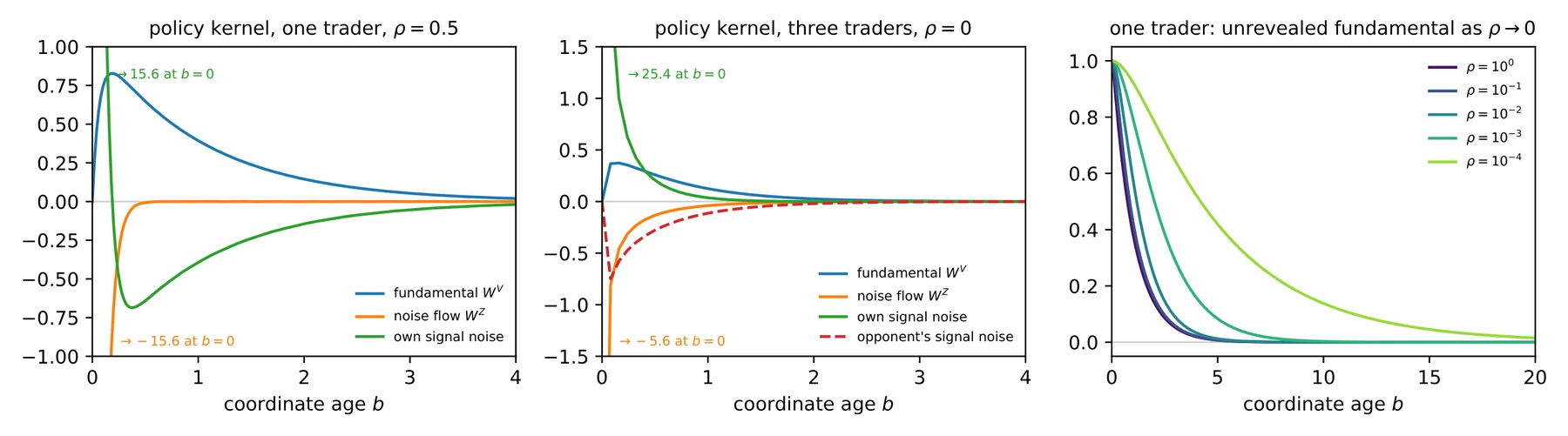
The unrevealed fundamental, the share of a fundamental shock not yet in the price by the shock’s age, is $0.39$ at age one with one trader and $0.25$ with three. A monopolist with a random-walk fundamental has no reason to trade its information by any particular date; its horizon comes from discounting, or, in Kyle’s model, from the terminal date. With an opponent, information not traded now is traded by the opponent, so the two- and three-trader solutions exist at $ρ = 0$ and reveal the shock by age two.

Table 4.1. Profit accounts of the symmetric markets ( $ρ = 0$ , $ϵ = 1 0^{- 3}$ ). Rates are flows per unit time; the book gap is a level. Each of the $N$ traders takes $λ Σ_{Z} / N$ of the traders’ row.
	price profits	execution	position	book gap, $N = 1, 2, 3$
traders, together	$+ λ Σ_{Z}$	$0$	$+ λ Σ_{Z}$	$0.06, 0.36, 0.29$
noise traders	$- λ Σ_{Z} /2$	$+ λ Σ_{Z} /2$	$- λ Σ_{Z}$	$- 0.06, - 0.36, - 0.29$
market maker	$- λ Σ_{Z} /2$	$- λ Σ_{Z} /2$	$0$	$0$

Symmetry forces the accounts (Table 4.1): each trader takes $λ Σ_{Z} / N$ , all of it position, and the noise traders take half of what they pay back as execution. The monopolist’s gap is the trading-cost residual, $2 ϵ / ρ$ to leading order: its undervalued fundamental positions, worth $+ 0.50$ at every cost, net exactly at zero cost against the overvalued positions it holds on its own signal noise. The monopolist holds those own-noise positions without buying any gap on them: its gap purchases on its own signal noise are zero. The competitors’ gaps do not shrink with the cost. A competitor trades the current signal immediately, buys $0.34$ of overvaluation on its own noise, and recovers $0.20$ on the others’. Table 4.2 varies the common signal gain of two traders.

Table 4.2. One of two symmetric traders’ book gap by channel as the common signal gain varies ( $ρ = 0$ , $ϵ = 1 0^{- 3}$ , window scaled with the trading speed). Every channel and the net scale together with the half-profit age, as $1/ γ$ . The competitors’ gap is the edge withheld from opponents. Per-trader price profits are $0.50$ at every gain, and the gap, unlike the monopolist’s $2 ϵ / ρ$ , does not shrink with the trading cost.
	$γ = 0.25$	$0.5$	$1$	$2$	$4$
half-profit age	1.36	0.68	0.34	0.18	0.10
fundamental book	$+ 0.81$	$+ 0.40$	$+ 0.20$	$+ 0.10$	$+ 0.05$
noise-trader book	$+ 0.46$	$+ 0.23$	$+ 0.12$	$+ 0.06$	$+ 0.03$
own-noise book	$- 1.37$	$- 0.68$	$- 0.34$	$- 0.17$	$- 0.08$
opponent-noise book	$+ 0.82$	$+ 0.41$	$+ 0.20$	$+ 0.10$	$+ 0.05$
net book gap	$0.72$	$0.36$	$0.18$	$0.09$	$0.05$

Competition also changes whose flow pays the trader: the monopolist’s position profits come entirely from its own flow moving the price, while with opponents each trader earns $0.72$ from its own flow and loses $0.22$ to its opponents’ (spectral values at $ϵ = 1 0^{- 3}$ ). On the shared channels, the fundamental and the noise-trader flow, an opponent’s flow pays a book exactly as the trader’s own does (Table 4.3). The tax falls on the private channels: a trader marks up its own noise-driven positions with its later orders, and its opponent, which does not share the noise, trades against exactly those price moves. Opponents charge a trader for the errors its noise puts into the price; the monopolist escapes because its own-noise purchases are zero.

Table 4.3. Position profits of one of two symmetric traders, by shock channel and by whose flow moves the price (spectral solution, $ϵ = 1 0^{- 3}$ ). The shared channels pay from either flow equally; the opponents’ tax is confined to the private noise channels.
	own flow	opponents’ flow
fundamental	$+ 0.125$	$+ 0.125$
noise-trader flow	$+ 0.125$	$+ 0.125$
own signal noise	$+ 0.235$	$- 0.441$
opponent’s signal noise	$+ 0.235$	$- 0.029$
total	$+ 0.720$	$- 0.220$

4.8.5Two assets

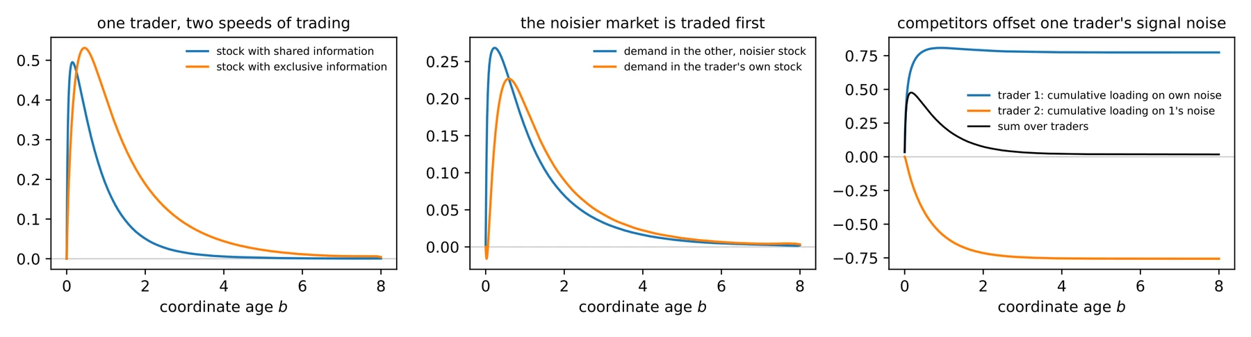
The two-asset equilibria, each with two traders at trading cost $2 \times 1 0^{- 3}$ and discount rate $ρ = 0.1$ , are computed in three configurations, the last two with fundamental correlation $0.6$ : signal gains $(1, 1)$ for both traders in the symmetric case with $Σ_{V} = I$ ; gains $(1, 1)$ and $(1, 0)$ in the generalist–specialist market; gains $(1, 0)$ and $(0, 1)$ with noise-trader variance $diag (1.8, 0.2)$ in the specialist case. A trader holding exclusive information in one market and shared information in the other trades them at different speeds, and a specialist whose own market has little noise-trader flow trades its information first in the other market, where that flow is larger (Figure 4.4). The instantaneous impact $Λ$ is a matrix across assets: in the symmetric case it is $1.001$ on the diagonal with no cross-impact, while in the specialist case the off-diagonal entries reach $0.42$ , so an order in one asset moves the other’s price.

Figure 4.4. Two-asset equilibria at trading cost $2 \times 1 0^{- 3}$ . Left: one trader, two market structures, two speeds of trading. Center: the trade in the market with more noise-trader flow comes first. Right: competitors’ trades offset one trader’s signal noise, so the sum over traders returns to zero.

4.8.6Deviation impact

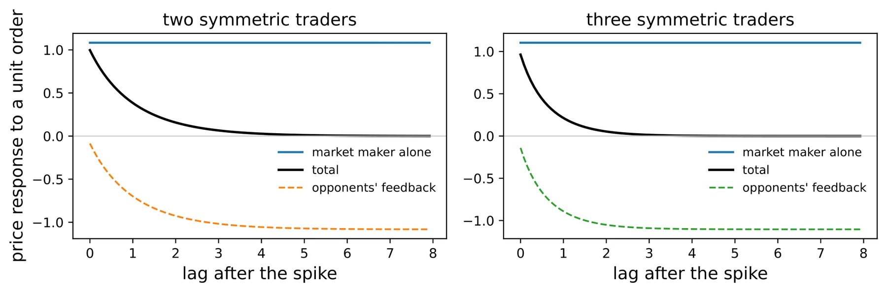
The impact of a deviation is not the pricing kernel, the market maker’s permanent price response to a unit of unexpected order flow. Figure 4.5 splits the price response to a unit order at age zero, the kernel $p_{i} (τ, t; z)$ of (4.4.14), into the market maker’s own update and the opponents’ feedback, by re-running the forward response of Section 4.4 with the opponents’ policies switched off (two and three symmetric traders, $ϵ = 0.1$ , $ρ = 0.1$ ). The market maker alone moves the price permanently, by $1.08$ per unit. The opponents see order flow that is not theirs and no news in their own signals, so they sell against it. On impact they absorb $8$ percent of the move with one opponent and $13$ percent with two. Afterwards they unwind all of it, half by ages $0.72$ and $0.48$ and everything by age eight. The instantaneous impact is $λ$ , but the discounted execution cost in the first-order condition, $\int_{t}^{\infty} e^{- ρ (τ - t)} D_{τ} p_{i} (τ, t; z) d τ$ , is a fraction of what the permanent response alone would imply, and the fraction falls with competition. In the generalist–specialist market a unit order in the shared stock is absorbed $14$ percent on impact and unwound on the same clock.

Figure 4.5. Price response to a unit order by one trader at age zero, decomposed by re-running the forward response with the opponents’ policies switched off ( $ϵ = 0.1$ , $ρ = 0.1$ ; the large cost smooths the kernels, and the decomposition is about shape). The market maker alone moves the price permanently; the opponents trade against the order and unwind the move, so the total response is transitory even though the pricing kernel is not.

4.8.7Asymmetric noise

Three traders with correlated fundamentals and asymmetric noise-trader flow separate two roles that the symmetric cases merge. Table 4.4 lists the parameters; Tables 4.5 and 4.6 report price profits and impact. Price discovery does not depend on $ζ$ : the unrevealed fundamental at ages one and two is $0.20$ and $0.04$ , at every $ζ$ . Price profits do. As stock two’s noise-trader flow shrinks, the quiet-stock leader’s price profits fall from $0.66$ to $0.39$ and the noisy-stock leader’s rise from $0.66$ to $0.81$ ; the generalist loses a little, $0.53$ to $0.48$ . These price profits are net of the trading cost, and Table 4.7’s totals are gross, $0.01$ to $0.02$ higher for the heavier traders. The quiet stock’s leader takes its information to the noisy stock: at $ζ = 0.8$ it trades its own factor in the noisy stock with integrated loading $0.19$ against $0.28$ in its own, up from $0.07$ against $0.64$ at $ζ = 0$ . Impact follows the noise: at $ζ = 0.8$ the own impact is $0.73$ in the noisy stock and $2.01$ in the quiet one. The cross-impact is asymmetric because the quiet stock’s flow is the more informative: an order in the quiet stock moves the noisy stock’s price by $0.45$ , while an order in the noisy stock moves the quiet stock’s by $0.31$ . Every trader runs two clocks: its loading on its own factor peaks by age $0.24$ , and its hedge against the correlated factor, traded in the opposite direction, peaks between ages $0.6$ and $1$ .

Table 4.4. Parameters of the three-trader asymmetric-noise market.
fundamentals	two, correlation $0.6$
signal gains (stock one, stock two)	trader one $(1.5, 0.5)$ , trader two $(0.5, 1.5)$ ,generalist $(1, 1)$
noise-trader variances	$diag (1 + ζ, 1 - ζ)$ , $ζ = 0, 0.5, 0.8$
discount rate, trading cost	$ρ = 0$ , $ϵ = 2 \times 1 0^{- 3}$ (halving it moves the numbers by about two percent)
window, collocation	$L = 16$ , $64$ Chebyshev points

Table 4.5. Price profits net of the trading cost in the three-trader market with noise-trader variances $diag (1 + ζ, 1 - ζ)$ ; in parentheses, the part earned in the noisy stock.
	$ζ = 0$	$ζ = 0.5$	$ζ = 0.8$
noisy-stock leader	0.66(0.57)	0.76(0.70)	0.81(0.77)
quiet-stock leader	0.66(0.09)	0.52(0.12)	0.39(0.14)
generalist	0.53(0.26)	0.51(0.33)	0.48(0.36)

Table 4.6. Entries of the matrix $Λ$ in the same market.
	$ζ = 0$	$ζ = 0.5$	$ζ = 0.8$
own impact, noisy stock	0.94	0.79	0.73
own impact, quiet stock	0.94	1.31	2.01
quiet-stock order on the noisy price	0.31	0.36	0.45
noisy-stock order on the quiet price	0.31	0.30	0.31

Table 4.7. Profit accounts in the three-trader market at $ζ = 0.8$ , by stock (spectral solution, $ϵ = 2 \times 1 0^{- 3}$ ). Position profits split into the part earned by the trader’s own flow and the part its opponents’ flow takes back; the total is price profits over both stocks. The gap is a level, not a flow, so it does not enter the total. Rates are flows per unit time. Each column is zero-sum, and the market maker’s position profits and book gap are zero stock by stock, up to the trading cost.
	noisy stock			quiet stock
	execution
(own/opponents’)	gap	execution
(own/opponents’)	gap	total

leader	0.00	$+ 0.79$ $(+ 1.08/ - 0.28)$	$+ 0.23$	0.00	$+ 0.04$ $(+ 0.06/ - 0.02)$	$+ 0.01$	$+ 0.83$

leader	0.00	$+ 0.14$ $(+ 0.24/ - 0.10)$	$+ 0.03$	0.00	$+ 0.25$ $(+ 0.34/ - 0.08)$	$+ 0.08$	$+ 0.40$
generalist	0.00	$+ 0.38$ $(+ 0.60/ - 0.22)$	$+ 0.11$	0.00	$+ 0.12$ $(+ 0.18/ - 0.07)$	$+ 0.04$	$+ 0.49$
noise traders	$+ 0.66$	$- 1.31$	$- 0.37$	$+ 0.20$	$- 0.40$	$- 0.12$	$- 0.86$
market maker	$- 0.66$	$- 0.01$	$0.00$	$- 0.20$	$0.00$	$0.00$	$- 0.86$

Symmetry no longer forces the accounts; Table 4.7 gives them at $ζ = 0.8$ . On the home books the clock is common: the ratio of book gap to position profits is $0.28$ – $0.32$ for each trader’s home stock, the generalist, and the noise traders, at every $ζ$ , so the noise asymmetry redistributes who buys undervaluation, not how long the price takes to pay it out. The specialists’ small cross-stock books turn over faster, $0.19$ – $0.26$ . Opponents tax the generalist hardest: the specialists lose a quarter to three tenths of their own-flow position profits to opponents’ trades, the generalist more than a third, its errors being visible to both specialists. The quiet stock’s leader earns seven tenths as much from its own flow in the noisy stock as at home, up from a fifth at $ζ = 0$ . The noise traders in the quiet stock lose $2.01$ in position per unit of their variance against $0.73$ in the noisy one, the net impacts $Λ_{22}$ and $Λ_{11}$ .

4.8.8The three terms of the order

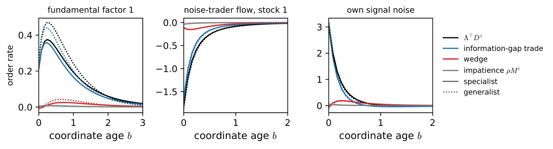
Theorem 4.10 splits each trader’s order into the information-gap trade, impatience, and the wedge (Figure 4.6, computed on the lag grid). The information-gap trade carries $92$ percent of the order, in $L^{2}$ norm over the policy kernels, in every case computed. Under the unbiasedness that the solutions satisfy, it is $E [D_{t}^{tot} ∣ F_{t}^{i}]$ , so the wedge is the price-impact value of the opponents’ expected current orders with the sign reversed, $- Λ E [D_{t}^{- i} ∣ F_{t}^{i}]$ ( $Λ$ is symmetric in these runs), less impatience. A trader shades its order by what it expects the others to send. The wedge is $13$ percent of the order and lives at ages under two; impatience is $4$ percent in the $ρ = 0.1$ case and absent at $ρ = 0$ .

Figure 4.6. The three terms of Theorem 4.10 for each trader’s order in stock one, by coordinate age and shock channel, in the generalist–specialist market at $ρ = 0.1$ : specialist solid, generalist dotted. The right panel shows each trader’s own signal-noise channel.

4.8.9Numerical identities

The solutions satisfy, up to the size of the trading cost, several identities that the equations do not impose directly. Each trader’s policy kernel has zero projection onto the market maker’s information (relative norm below $5 \times 1 0^{- 3}$ at $ϵ = 1 0^{- 3}$ ). Summing over traders, total order flow is a Brownian motion in the market maker’s own filtration, which extends the unbiasedness that Back [11] proved for a single trader to every case computed here. The pricing kernel is constant across ages to within $0.2$ percent, so each unexpected unit of order flow moves the price permanently and by the same amount at every age. The sum over ages of total trader demand’s loading on each signal noise is zero. Competitors fully offset one another’s noise-driven positions, while a monopolist has no one to offset them and is left with a net position of $1 0^{- 3}$ , the size of the cost. Total price profits gross of the trading cost equal the noise traders’ position losses $λ Σ_{Z}$ to $2 \times 1 0^{- 4}$ for one, two, and three traders, and do not depend on the lag truncation $L$ of Appendix 4.A. The net price profits fall short by exactly the cost, $0.006$ per trader with two or three traders. As the cost vanishes, each competitor’s loading on its own signal noise at age zero grows like $ϵ^{- 1/2}$ while its integral stays fixed, so the loading is concentrated on ages of order $ϵ^{1/2}$ and the net shortfall falls like $ϵ^{1/2}$ . In the limit a competitor trades its current signal noise as an impulse, and total price profits equal $λ Σ_{Z}$ exactly. Computed down to $ϵ = 5 \times 1 0^{- 5}$ , total price profits are $0.998$ . For one trader $λ$ and the price profits are $1.000$ , the values of Back’s continuous-time equilibrium. Proofs of these identities are open.

4.AComputing the Kyle–Back equilibria

The equilibria of Section 4.8 are fixed points of the joint best-response map over all traders’ kernels, computed by Newton’s method on the difference between a profile and its best response, with the cost $ϵ$ continued downward from a large value at which the map is well conditioned. Damped best-response iteration fails here. The equilibrium is unstable under it, with the dominant eigenvalue of the best-response map above one. More trading raises price impact, higher impact reduces trading, and less trading lowers impact again, so the iteration oscillates instead of converging. Newton iteration does not depend on this stability and converges to residuals near $1 0^{- 10}$ in a few steps.

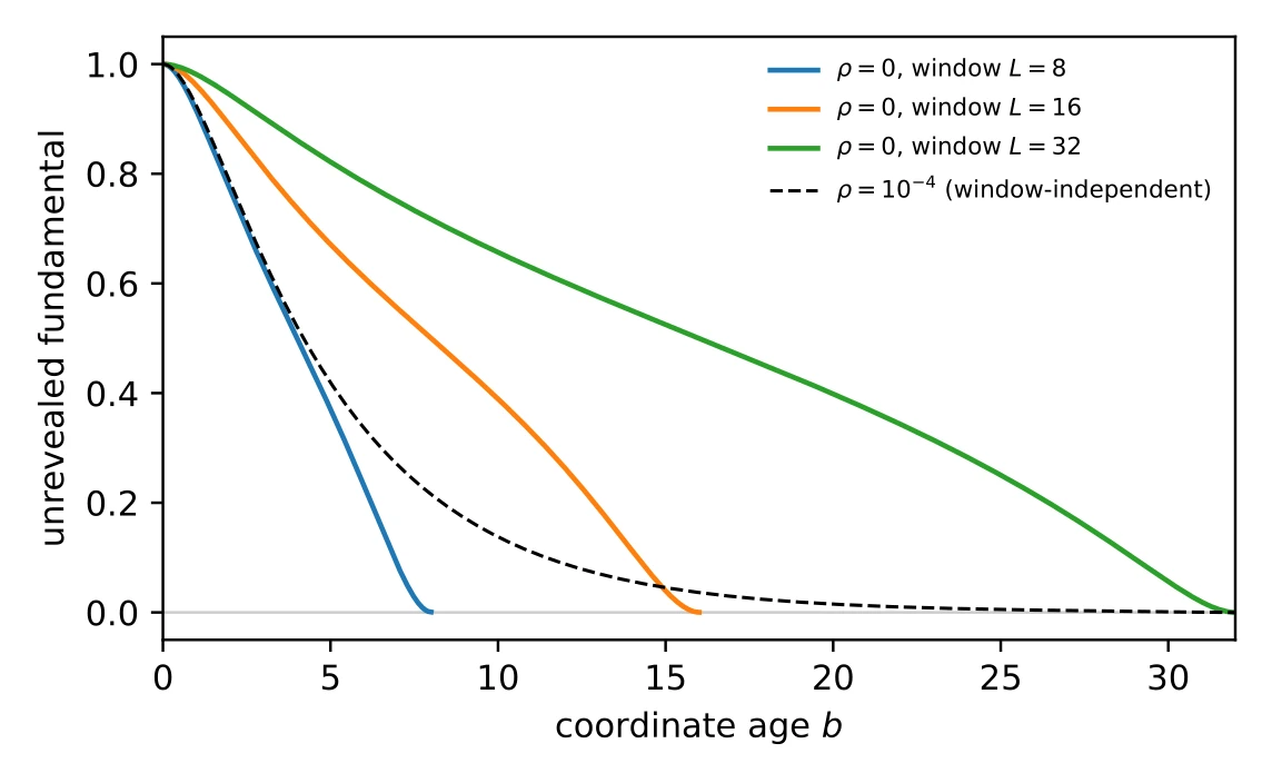
The computations use the average-cost objective ( $ρ = 0$ ) with lags truncated at $L = 8$ as in Chapter 3; the window replaces the transversality of Assumption 4.1, and its effect is measured below. The kernels are represented by their values at 64 Chebyshev points on $[0, L]$ by the spectral collocation of Appendix 3.A. The three-trader scalars are unchanged to four digits at 96 and 128 points. The two-asset equilibria use the same solver in its two-asset form; the three-trader asymmetric-noise market runs with $L = 16$ and $ϵ = 2 \times 1 0^{- 3}$ , and its profit accounts are computed from the node values by Chebyshev quadrature, with positions as spectral antiderivatives. The window must scale with the half-profit age, so the gain ladder of Table 4.2 uses windows up to $L = 32$ . The loading on own signal noise carries an impulse of width $ϵ^{1/2}$ at age zero, and at 64 points the collocation solution rings behind it, a node-to-node alternation of $3 \times 1 0^{- 3}$ in the tail. At 128 points the alternation is $2 \times 1 0^{- 4}$ , and the three-trader kernels of Figure 4.3 are drawn from that solution. With two or more traders the fundamental is essentially fully revealed well before age $L$ and the reported quantities do not depend on it. The two- and three-trader kernels agree at $L = 8$ and $L = 16$ to four digits beyond age one. A single undiscounted trader has no such solution. Its kernels scale with $L$ , half of its profit accrues after age $0.19 L$ , and the unrevealed fundamental falls to zero exactly at $L$ . The truncation plays the part of Kyle’s terminal date: the undiscounted computation converges on a window only because the window supplies the terminal date. Figure 4.7 shows the artifact. With a discount rate $ρ > 0$ the one-trader solution is the same at $L = 8$ , $16$ , and $32$ . As $ρ$ falls (Figure 4.3, right) the horizon, measured as one over the share revealed by age one, grows without bound and approaches the rate $ρ^{- 1/2}$ ( $1.63$ , $1.75$ , $2.37$ , $4.88$ , $13.1$ at $ρ = 1, 1 0^{- 1}, \dots, 1 0^{- 4}$ ). The scalars are unaffected: $λ$ , total price profits, and the channel split are the same at every $ρ$ . The second-order checks are made on the average-cost system and do not rely on the $ρ > 0$ hypothesis of Assumption 4.1. The market maker’s belief update is computed as in Appendix 3.A.

Figure 4.7. The window artifact for one undiscounted trader: the unrevealed fundamental by shock age computed at $ρ = 0$ on windows $L = 8$ , $16$ , and $32$ falls linearly to zero exactly at $L$ , so each window gives a different solution. The discounted solution at $ρ = 1 0^{- 4}$ (dashed) is the same on every window.

Every reported solution has passed the second-order check of Section 4.8 and a comparison between solvers. The spectral solver reproduces the grid solver’s extrapolations to zero spacing.

On a lag grid, how price impact is timed within an interval matters more than how fine the spacing is. If the scheme realizes the price impact at the midpoint of the interval, a trader can buy and later sell the same quantity at a profit that comes entirely from the half-interval delay between an order and its own impact. The second-order condition fails below a cost threshold proportional to the spacing. Realizing the impact within the same interval as the order removes that profit. The spectral solver works in continuous lag, where an order’s impact arrives with the order and a round trip under permanent impact pays only the trading cost. It therefore reports the small-cost equilibria.

The solvers and figures of Section 4.8 are the work of Claude Fable 5 [7], working under the author’s direction. Interactive versions are at sbabichenko.com/noisestate.