Chapter 3Stationary Infinite-Horizon LQG

In the finite-horizon chapter every kernel depends on two calendar dates, the source date of a shock and the date of its evaluation. Here the calendar drops out and only ages remain, the age of the shock and the age of the belief about it. The causal triangle of Chapter 1 becomes a lag quadrant, the quarter plane of two nonnegative ages.

The stationary case matters for four reasons. First, every impulse response function becomes time invariant, and a simple recipe turns the identities of Chapter 1 into stationary ones. The stationary system is therefore easier to compute and plot. Most work building on these methods would study stationary cases. An economic system that has settled into stationary equilibrium under one policy, like the economy behind an estimated Phillips curve, begins any new regime from that stationary state. The response to the shift is a nonstationary problem, so studying a regime change means solving the stationary problem first. Second, much of the literature studies the stationary case through the frequency domain [60, 64, 101], so working in the stationary case makes comparisons easier. Third, the stationary case makes it easier to see how close the system is to Markovian. A stationary linear Markov process has impulse responses that are combinations of exponentials, so how well such combinations fit the kernels here measures how far the equilibrium is from finite-dimensional. Finally, this chapter is the setting of the Kyle–Back analysis. The stationary deviation calculus of Chapter 4 runs in the lag coordinates introduced here, and its equilibrium condition plays the role of Proposition 3.1.

3.1Stationary profiles, lag coordinates, and forward filtering

The time-homogeneous primitives are $d X_{t} d Y_{t}^{i} d Z_{t} = (B_{X}^{X} X_{t} + m = 1 \sum n B_{m}^{X} D_{t}^{m} + m = 1 \sum n \tilde{B}_{m}^{X} D_{t - τ_{m}}^{m}) d t + σ d W_{t}^{0}, = (B_{X}^{Y, i} X_{t} + m = 1 \sum n B_{m}^{Y, i} D_{t -}^{m}) d t + E^{i} d W_{t}, i = 1, \dots, n, = (B_{X}^{Z} X_{t} + m = 1 \sum n B_{m}^{Z} D_{t -}^{m}) d t + E^{Z} d W_{t} . (3.1.1) (3.1.2) (3.1.3)$ Two delays are allowed. A control may act on the state after a lag $τ_{m} \geq 0$ (the $\tilde{B}_{m}^{X}$ rows; $D_{s}^{m} := 0$ for $s < 0$ ). The public signal $Z$ is observed by player $i$ with delay $Δ_{i} \geq 0$ , so that $F_{t}^{i} = σ (Y_{r}^{i} : r \leq t) \lor σ (Z_{r} : r \leq t - Δ_{i})$ , with the rows normalized and orthogonal as in Chapter 2: $E^{i} E^{i ⊤} = I$ , $E^{Z} E^{Z ⊤} = I$ , $E^{i} E^{Z ⊤} = 0$ . Private rows may also carry other players’ predictable controls (observed actions, $B_{m}^{Y, i}$ ). Setting $\tilde{B}_{m}^{X} = 0$ , $B_{m}^{Y, i} = 0$ and dropping $Z$ recovers the baseline. Here $W = (W^{0}, W^{1}, \dots, W^{n})$ , $Π^{i} = E^{i ⊤} E^{i}, P^{i} = (B_{X}^{Y, i})^{⊤} B_{X}^{Y, i} .$ Player $i$ ’s discounted objective is

$J^{i} = \frac{1}{2} E \int_{0}^{\infty} e^{- ρt} [X_{t}^{⊤} G^{XX, i} X_{t} + 2 (G^{X, i})^{⊤} X_{t} + 2 (D_{t}^{i})^{⊤} G^{D X, i} X_{t} + (D_{t}^{i})^{⊤} G^{DD, i} D_{t}^{i}] d t, ρ > 0, (3.1.4)$

with the joint running Hessian positive semidefinite.

All lags are calendar time minus source time: $a = t - s \geq 0, b = t - u \geq 0, ℓ = t - s \in R . (3.1.5)$ Delays are fixed ages. The variables $a, b$ are ages of past state and noise-state coordinates. The adjoint lag $ℓ$ is two-sided; future source times have $ℓ < 0$ . Brownian motions are extended to two-sided time for adjoint formulas.

The front-matter Notation reference collects the finite-horizon-to-stationary translation. Every lowercase object below is the corresponding Chapter 1 object after calendar time drops out. For adjoints the lowercase kernel is the current-value form, $h^{X, i} (t - s) := e^{ρt} H_{t}^{X, i} (s)$ and $h^{k, i} (t - u, t - s) := e^{ρt} H_{t}^{k, i} (u, s)$ , which is why $ρ h$ appears in (3.2.9) in place of the finite-horizon time derivative.

A stationary noise-state linear profile has $D_{t}^{i} = \overset{ˉ}{d}^{i} + \int_{0}^{\infty} d^{i} (a) d W_{t}^{i} (a), d W_{t}^{i} (a) := d E [W_{t - a} ∣ F_{t}^{i}] . (3.1.6)$ The same weight $d^{i} (a)$ applies at every date to the player’s belief about a shock of age $a$ . With the delayed public row the noise-state has the representation of Chapter 2 in age form, $d W_{t}^{i} (a) = Π^{i} d W_{t - a} + 1_{{a > Δ_{i}}} Π^{Z} d W_{t - a} + (\int_{0}^{\infty} f^{i} (a, b) d W_{t - b} d b) d a$ , with $Π^{Z} = E^{Z ⊤} E^{Z}$ and $f^{i} (a, b)$ the kernel from the coordinate of age $a$ to the source of age $b$ . Shocks older than the delay are also known through their public increment. The profile is admissible if the displayed integrals are square-integrable, the induced filtering operators are bounded, and the closed-loop response kernels below decay fast enough for the discounted cost to be finite and all integration-by-parts identities to hold. The discounted boundary terms generated by integration by parts vanish at long horizons, which is the transversality used in Proposition 3.1. A stationary equilibrium in this class is a stationary profile for which no player can reduce (3.1.4) by a unilateral stationary noise-state linear deviation.

The finite-horizon state-response equation $\partial_{t} X_{t} (s) = B_{X}^{X} X_{t} (s) + m = 1 \sum n B_{m}^{X} D_{W, t}^{m} (s), X_{s} (s) = (σ, 0, \dots, 0) (3.1.7)$ becomes, with $X_{t} (s) = x (t - s)$ and $D_{W, t}^{m} (s) = d_{W}^{m} (t - s)$ ,

$x^{'} (a) = B_{X}^{X} x (a) + m = 1 \sum n B_{m}^{X} d_{W}^{m} (a) + m = 1 \sum n \tilde{B}_{m}^{X} 1_{{a \geq τ_{m}}} d_{W}^{m} (a - τ_{m}), x (0) = (σ, 0, \dots, 0), x (a) \to 0. (3.1.8)$

The stationary mean satisfies $0 = B_{X}^{X} \overset{ˉ}{X} + m = 1 \sum n B_{m}^{X} \overset{ˉ}{d}^{m} + m = 1 \sum n \tilde{B}_{m}^{X} \overset{ˉ}{d}^{m} . (3.1.9)$ For filter kernels $F_{t}^{i} (u, s) = f^{i} (b, a)$ , so $\partial_{t} = \partial_{b} + \partial_{a}$ . For adjoint kernels $H_{t} (s) = h (ℓ)$ , so $\partial_{t} = \partial_{ℓ}$ ; with a noise-state coordinate $b = t - u$ , the transport derivative is $\partial_{b} + \partial_{ℓ}$ .

Each instant a new shock is born unknown and every old shock is known a little better, so each shock’s uncertainty falls over its lifetime while the cross-section of uncertainty over ages stays fixed.

The control kernel in primitive-shock coordinates is $d_{W}^{i} (a) = d^{i} (a) (Π^{i} + 1_{{a > Δ_{i}}} Π^{Z}) + \int_{0}^{\infty} d^{i} (b) f^{i} (b, a) d b . (3.1.10)$ This carries the policy kernel $d^{i}$ into primitive coordinates: how player $i$ ’s control answers a shock of age $a$ . The unresolved state response is $\tilde{x}^{i} (a) = x (a) (I - Π^{i} - 1_{{a > Δ_{i}}} Π^{Z}) - \int_{0}^{\infty} x (b) f^{i} (b, a) d b . (3.1.11)$ This is the state’s response to a shock less the part player $i$ has already resolved, privately or through the public row. The private row’s drift kernel is $c^{i, Y} (a) = B_{X}^{Y, i} x (a) + \sum_{m} B_{m}^{Y, i} d_{W}^{m} (a)$ and its unresolved part $\tilde{c}^{i, Y} (a) = c^{i, Y} (a) (I - Π^{i} - 1_{{a > Δ_{i}}} Π^{Z}) - \int_{0}^{\infty} c^{i, Y} (b) f^{i} (b, a) d b$ ; without observed actions $\tilde{c}^{i, Y} = B_{X}^{Y, i} \tilde{x}^{i}$ . The delayed public row generated $Δ_{i}$ ago has drift kernel $c^{Z} (a) = B_{X}^{Z} x (a) + \sum_{m} B_{m}^{Z} d_{W}^{m} (a)$ at its source time; its centered innovation kernel at the arrival date is (Chapter 2, in ages) $\tilde{c}^{i, Z} (a) = c^{Z} (a - Δ_{i}) (I - Π^{i} - 1_{{a > Δ_{i}}} Π^{Z}) - \int_{0}^{\infty} c^{Z} (b - Δ_{i}) f^{i} (b, a) d b - E^{Z} f^{i} (Δ_{i}^{-}, a), (3.1.12)$ with $c^{Z} (b - Δ_{i}) := 0$ for $b < Δ_{i}$ (the row generated $Δ_{i}$ ago loads only on shocks that existed then). In the last term player $i$ subtracts what it had already inferred about the arriving public increment. The stationary filter is $(\partial_{b} + \partial_{a}) f^{i} (b, a) f^{i} (b, 0) f^{i} (0, a) f^{i} (b, Δ_{i})_{Z} = \tilde{c}^{i, Y} (b)^{⊤} \tilde{c}^{i, Y} (a) + \tilde{c}^{i, Z} (b)^{⊤} \tilde{c}^{i, Z} (a), b, a > 0, b, a \neq = Δ_{i}, = \tilde{c}^{i, Y} (b)^{⊤} E^{i}, b > 0, = E^{i ⊤} \tilde{c}^{i, Y} (a), a > 0, = \tilde{c}^{i, Z} (b)^{⊤} E^{Z}, f^{i} (Δ_{i}, a)_{Z} = E^{Z ⊤} \tilde{c}^{i, Z} (a), (3.1.13) (3.1.14) (3.1.15) (3.1.16)$ the last line being the second birth, at age $Δ_{i}$ , when the public news about a shock arrives, with $\cdot ∣_{Z}$ the $E^{Z}$ block. With $B_{m}^{Y, i} = 0$ the private source is $\tilde{x}^{i} (b)^{⊤} P^{i} \tilde{x}^{i} (a)$ and the births are $\tilde{x}^{i} (b)^{⊤} (B_{X}^{Y, i})^{⊤} E^{i}$ , $E^{i ⊤} B_{X}^{Y, i} \tilde{x}^{i} (a)$ . Equivalently, in the baseline, for $b \neq = a$ , $f^{i} (b, a) = f^{i} (b, a) = \tilde{x}^{i} (b - a)^{⊤} (B_{X}^{Y, i})^{⊤} E^{i} + \int_{0}^{a} \tilde{x}^{i} (b - c)^{⊤} P^{i} \tilde{x}^{i} (a - c) d c, E^{i ⊤} B_{X}^{Y, i} \tilde{x}^{i} (a - b) + \int_{0}^{b} \tilde{x}^{i} (b - c)^{⊤} P^{i} \tilde{x}^{i} (a - c) d c, b > a, a > b . (3.1.17) (3.1.18)$ The diagonal is a separate pointwise convention, $f^{i} (a, a) := f_{diag}^{i} (a), (3.1.19)$ and does not affect the integral equations.

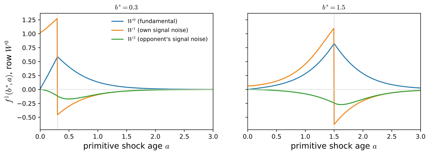
The numerical benchmark is the stationary form of the tracking example of Chapter 1. The state is scalar with $d X_{t} = (D_{t}^{1} + D_{t}^{2}) d t + d W_{t}^{0}$ , each player observes $d Y_{t}^{i} = p_{i} X_{t} d t + d W_{t}^{i}$ with $p_{1} = p_{2} = 3$ and effort weights $r_{1} = r_{2} = 0.1$ on $(D_{t}^{i})^{2}$ as in Chapter 1, and the objective is average cost. Section 3.2 also varies each precision from $1$ to $20$ with the other held at $3$ . Proposition 3.1 verifies the discounted system, so these computations give solutions of the formal average-cost stationary equations, the $ρ = 0$ form of that system, rather than a verified optimum. Figure 3.1 shows the resulting kernel, with one curve per primitive shock.

Figure 3.1. Decomposition by primitive shock of the $W^{0}$ channel of the stationary filter kernel $f^{1} (b^{*}, a)$ at two coordinate ages $b^{*}$ . The loading on the opponent’s signal noise is nonzero only because that noise moves the opponent’s actions and through them the state.

Figure 3.2. The stationary two-sided state price $h^{X, 1} (ℓ)$ in the symmetric two-player benchmark ( $p_{1} = p_{2} = 3$ , $r_{1} = r_{2} = 0.1$ , average cost), from the spectral solution with 32 Chebyshev points per side.

3.2Current-value adjoints

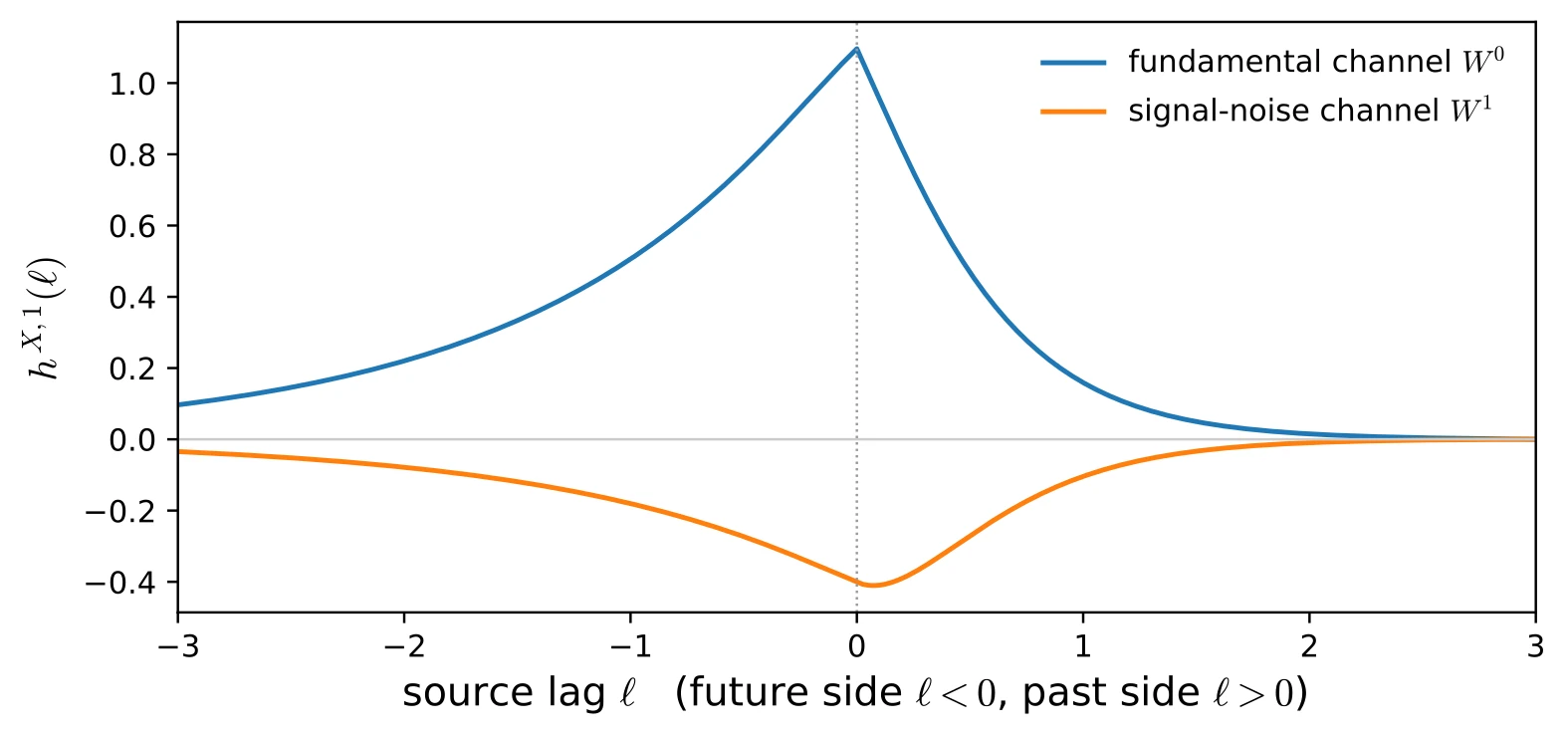
The unprojected state price is two-sided: $H_{t}^{X, i} = \overset{ˉ}{h}^{X, i} + \int_{- \infty}^{\infty} h^{X, i} (ℓ) d W_{t - ℓ} . (3.2.1)$ The player cannot act on future shocks, so the control uses the conditional expectation of this adjoint given $F_{t}^{i}$ : $D_{t}^{i} = - (G^{DD, i})^{- 1} E [G^{D X, i} X_{t} + (B_{i}^{X})^{⊤} H_{t}^{X, i} + e^{- ρ τ_{i}} (\tilde{B}_{i}^{X})^{⊤} H_{t + τ_{i}}^{X, i} + k \neq = i \sum (B_{i}^{Y, k})^{⊤} B^{k} H_{t}^{k, i} + k \neq = i \sum e^{- ρ Δ_{k}} (B_{i}^{Z})^{⊤} (B^{k, Z} H^{k, i})_{t + Δ_{k} \leftarrow t} F_{t}^{i}] . (3.2.2)$ In the last two sums player $i$ prices what its action does to opponent $k$ ’s beliefs: $H^{k, i}$ is its belief price on opponent $k$ ’s noise-state, and $B^{k}$ and $B^{k, Z}$ contract that price against $k$ ’s private and delayed-public filter rows, both defined immediately after (3.2.4). The subscript $_{t + Δ_{k} \leftarrow t}$ means a row generated at $t$ and evaluated on arrival at $t + Δ_{k}$ . In (3.2.2) and in the proof of Proposition 3.1, $H_{t}^{X, i}$ and $H_{t}^{k, i}$ are the current-value adjoint processes, $e^{ρt}$ times the costates of the discounted objective. Player $i$ prices a shock’s consequences through lags on both sides of the present. The negative lags show the benefit of acting on future shocks, and that benefit decays slowly with distance. The fundamental channel of $h^{X, 1}$ , its loading on the state noise, still holds a fifth of its peak at lag $ℓ = - 2$ , in the future, while at $ℓ = 2$ , in the past, it is nearly gone (Figure 3.2). The signal-noise channels, the loadings on the players’ signal noises, behave differently at the boundary. A noise shock harms only through the responses it triggers, and at arrival no player has responded to it yet, so the channels’ price peaks a short interval after the shock arrives. That near-boundary peak is the early peak. The peak lag shrinks as player 1’s own precision grows, since faster filtering corrects the belief error sooner, from lag $0.11$ at $p_{1} = 1$ to $0.02$ at $p_{1} = 20$ (Figure 3.3). The depth is not monotone in $p_{1}$ ; it is largest near $4$ . The opponent’s precision works the other way. A more precise opponent responds to the shock sooner and more accurately, so the price of the noise shock shrinks in magnitude, from $- 0.70$ at $p_{2} = 1$ to $- 0.12$ at $p_{2} = 20$ , and its peak moves later.

Figure 3.3. The early peak of $h^{X, 1}$ against precision: lag and depth of the minimum of the signal-noise channel as the observer’s own precision $p_{1}$ (solid) and the opponent’s $p_{2}$ (dashed) vary, the other held at $3$ . Two hundred equilibria per curve from the spectral solver.

Only lags $ℓ \geq 0$ are estimable at time $t$ , so

$\overset{ˉ}{d}^{i} d^{i} (a) = - (G^{DD, i})^{- 1} [G^{D X, i} \overset{ˉ}{X} + (B_{i}^{X} + e^{- ρ τ_{i}} \tilde{B}_{i}^{X})^{⊤} \overset{ˉ}{h}^{X, i} + k \neq = i \sum (B_{i}^{Y, k})^{⊤} B^{k} \overset{ˉ}{h}^{k, i} + k \neq = i \sum e^{- ρ Δ_{k}} (B_{i}^{Z})^{⊤} (B^{k, Z} \overset{ˉ}{h}^{k, i})], = - (G^{DD, i})^{- 1} [G^{D X, i} x (a) + (B_{i}^{X})^{⊤} h^{X, i} (a) + e^{- ρ τ_{i}} (\tilde{B}_{i}^{X})^{⊤} h^{X, i} (a + τ_{i}) + k \neq = i \sum (B_{i}^{Y, k})^{⊤} B^{k} h^{k, i} (a) + k \neq = i \sum e^{- ρ Δ_{k}} (B_{i}^{Z})^{⊤} (B^{k, Z} h^{k, i}) (a)], a > 0, (3.2.3)$

with the right trace $h^{X, i} (0^{+})$ used at $a = 0$ . Each term of (3.2.3) is an adjoint evaluated at the lag at which its effect occurs, and all are projected on $F_{t}^{i}$ . When player $i$ ’s action takes effect $τ_{i}$ later, the shock it reacts to now is $τ_{i}$ older, so the player reads the state price $τ_{i}$ further along the past-lag side; coordinates with age below $τ_{i}$ , noise born between action and effect, drop out. An action the opponent sees directly is priced now, by contracting the belief price against the opponent’s private filter row; an action that reaches the opponent only through the public signal is priced $Δ_{k}$ later, when that signal arrives.

For opponent $k \neq = i$ , write $H_{t}^{k, i} (b) = \overset{ˉ}{h}^{k, i} (b) + \int_{- \infty}^{\infty} h^{k, i} (b, ℓ) d W_{t - ℓ}, b \geq 0. (3.2.4)$ The values at $b = 0$ are right traces. Write the private and delayed-public contractions of a belief price against opponent $k$ ’s filter as $B^{k} h (ℓ) (B^{k, Z} h) (ℓ) := E^{k} h (0^{+}, ℓ) + \int_{0}^{\infty} \tilde{c}^{k, Y} (b) h (b, ℓ) d b, := E^{Z} h (Δ_{k}^{+}, ℓ + Δ_{k}) + \int_{0}^{\infty} \tilde{c}^{k, Z} (b) h (b, ℓ + Δ_{k}) d b .$ Define $\overset{v}{ˉ}^{k, i} v^{k, i} (ℓ) = (B_{X}^{Y, k})^{⊤} B^{k} \overset{ˉ}{h}^{k, i} + e^{- ρ Δ_{k}} (B_{X}^{Z})^{⊤} (B^{k, Z} \overset{ˉ}{h}^{k, i}), \overset{v}{ˉ}^{i} = k \neq = i \sum \overset{v}{ˉ}^{k, i}, = (B_{X}^{Y, k})^{⊤} B^{k} h^{k, i} (ℓ) + e^{- ρ Δ_{k}} (B_{X}^{Z})^{⊤} (B^{k, Z} h^{k, i}) (ℓ), v^{i} (ℓ) = k \neq = i \sum v^{k, i} (ℓ) . (3.2.5) (3.2.6)$ Without the public row or observed actions the first terms reduce to the baseline: birth term $(B_{X}^{Y, k})^{⊤} E^{k} h^{k, i} (0^{+}, ℓ)$ plus accumulated drift inference $P^{k} \int \tilde{x}^{k} (b) h^{k, i} (b, ℓ) d b$ . When player $i$ ’s own control enters opponent $k$ ’s private row ( $B_{i}^{Y, k} \neq = 0$ ) the deviation moves that row directly. Like the public-row term $B_{i}^{Z}$ , its price $(B_{i}^{Y, k})^{⊤} B^{k} h^{k, i}$ enters player $i$ ’s first-order condition above rather than the state price. The sums $\overset{v}{ˉ}^{i}$ and $v^{i}$ are the information wedge, the price of moving another player’s beliefs, now including what the delayed public news will reveal.

The mean adjoint equations are $0 \frac{d}{d b} \overset{ˉ}{h}^{k, i} (b) = ρ \overset{ˉ}{h}^{X, i} - (G^{XX, i} \overset{ˉ}{X} + G^{X, i} + G^{X D, i} \overset{ˉ}{d}^{i}) - (B_{X}^{X})^{⊤} \overset{ˉ}{h}^{X, i} - \overset{v}{ˉ}^{i}, = ρ \overset{ˉ}{h}^{k, i} (b) - ((B_{k}^{X} + e^{- ρ τ_{k}} \tilde{B}_{k}^{X}) d^{k} (b))^{⊤} \overset{ˉ}{h}^{X, i} + r^{k, Y} (b)^{⊤} B^{k} \overset{ˉ}{h}^{k, i} + c^{Z} (b - Δ_{k})^{⊤} B^{k, Z} \overset{ˉ}{h}^{k, i} - k^{'} \neq = i \sum e^{- ρ Δ_{k^{'}}} (B_{k}^{Z} d^{k} (b))^{⊤} B^{k^{'}, Z} \overset{ˉ}{h}^{k^{'}, i}, \overset{ˉ}{h}^{k, i} (b) \to 0. (3.2.7) (3.2.8)$ Set $x_{+} (ℓ) = 1_{ℓ \geq 0} x (ℓ)$ and $d_{W, +}^{i} (ℓ) = 1_{ℓ \geq 0} d_{W}^{i} (ℓ)$ . Away from $ℓ = 0$ , $\partial_{ℓ} h^{X, i} (ℓ) (\partial_{b} + \partial_{ℓ}) h^{k, i} (b, ℓ) = ρ h^{X, i} (ℓ) - G^{XX, i} x_{+} (ℓ) - G^{X D, i} d_{W, +}^{i} (ℓ) - (B_{X}^{X})^{⊤} h^{X, i} (ℓ) - v^{i} (ℓ), h^{X, i} (ℓ) \to 0 (∣ ℓ ∣ \to \infty), = ρ h^{k, i} (b, ℓ) - (B_{k}^{X} d^{k} (b))^{⊤} h^{X, i} (ℓ) - e^{- ρ τ_{k}} (\tilde{B}_{k}^{X} d^{k} (b))^{⊤} h^{X, i} (ℓ + τ_{k}) + r^{k, Y} (b)^{⊤} B^{k} h^{k, i} (ℓ) + c^{Z} (b - Δ_{k})^{⊤} (B^{k, Z} h^{k, i}) (ℓ - Δ_{k}) - k^{'} \neq = i \sum e^{- ρ Δ_{k^{'}}} (B_{k}^{Z} d^{k} (b))^{⊤} (B^{k^{'}, Z} h^{k^{'}, i}) (ℓ), (3.2.9) (3.2.10)$ where $r^{k, Y} (b) = c^{k, Y} (b) - B_{k}^{Y, k} d^{k} (b)$ is the old-history coefficient of opponent $k$ ’s private row (the opponent’s own control is removed because its response to its beliefs is priced through $d^{k}$ ). In the baseline $r^{k, Y} (b)^{⊤} B^{k} h^{k, i} = x (b)^{⊤} v^{k, i}$ . Opponent $k$ ’s delayed control moves the state $τ_{k}$ later, so player $i$ prices that response at $ℓ + τ_{k}$ . The delayed public signal enters twice. Opponent $k$ now reads the public increment generated $Δ_{k}$ ago, which loads on the coordinate through $c^{Z} (b - Δ_{k})$ ; player $i$ prices it with the contraction at arrival, $(B^{k, Z} h^{k, i}) (ℓ - Δ_{k})$ . The row generated now carries opponent $k$ ’s response $B_{k}^{Z} d^{k} (b)$ and is observed by every opponent $k^{'}$ at $t + Δ_{k^{'}}$ , priced by $e^{- ρ Δ_{k^{'}}} (B^{k^{'}, Z} h^{k^{'}, i}) (ℓ)$ . At the arrival age $b = Δ_{k}$ the belief price jumps by the centering trace, $h^{k, i} (Δ_{k}^{-}, ℓ) - h^{k, i} (Δ_{k}^{+}, ℓ) = - E^{Z ⊤} [E^{Z} h^{k, i} (Δ_{k}^{+}, ℓ) + \int_{0}^{\infty} \tilde{c}^{k, Z} (b) h^{k, i} (b, ℓ) d b], (3.2.11)$ the stationary form of the jump condition (2.4.32) at the arrival date. The belief price $h^{k, i} (b, ℓ)$ decays as $b \to \infty$ and $∣ ℓ ∣ \to \infty$ .

Proposition 3.1 (Stationary verification). Fix a stationary admissible profile. Suppose its kernels satisfy the forward equations (3.1.8)–(3.1.19), the adjoint equations (3.2.5)–(3.2.10), the jump condition (3.2.11), the first-order condition (3.2.2), and the stated decay/transversality conditions. Then the profile is a stationary best response for each player in the noise-state linear class. If the Schur complement $S^{i} = G^{DD, i} - G^{D X, i} (G^{XX, i})^{+} G^{X D, i} ⪰ λ I$ for some $λ > 0$ ( $G^{D X, i} = 0$ is the tracking case, where $S^{i} = G^{DD, i}$ ), the stationary best response is unique.

Proof. Apply the discounted spike variation of Appendix 1.B.2 on $[0, T]$ with opponents’ stationary maps fixed, and let $T \to \infty$ . The limit is taken as the definition of the stationary problem, with the two-sided adjoints (3.2.1) the objects verified against; convergence of the finite-horizon adjoints to them is not proved here. Write the kernels of (1.B.10) in lag coordinates and in current value. The first variation of $J^{i}$ in a direction $z$ is then $δ J^{i} = E \int_{0}^{T} e^{- ρt} z_{t}^{⊤} (G^{DD, i} D_{t}^{i} + G^{D X, i} X_{t} + (B_{i}^{X})^{⊤} H_{t}^{X, i} + e^{- ρ τ_{i}} (\tilde{B}_{i}^{X})^{⊤} H_{t + τ_{i}}^{X, i} + k \neq = i \sum (B_{i}^{Y, k})^{⊤} B^{k} H_{t}^{k, i} + k \neq = i \sum e^{- ρ Δ_{k}} (B_{i}^{Z})^{⊤} (B^{k, Z} H^{k, i})_{t + Δ_{k} \leftarrow t}) d t$ plus boundary terms. The finite-horizon adjoints $\overset{ˉ}{H}_{t}^{X}$ , $H_{t}^{X} (\cdot)$ become the two-sided current-value adjoint (3.2.1), and (3.2.5)–(3.2.6) are the stationary form of the information wedge of Theorem 1.8. Integration by parts gives the boundary terms at age zero, at lag zero $ℓ = 0$ , at the arrival age $b = Δ_{k}$ , and at $T$ . The boundary terms at age zero are the axis birth terms (3.1.14)–(3.1.15); the terms at $ℓ = 0$ cancel because bounded sources keep the kernels continuous there; the terms at the arrival age $b = Δ_{k}$ are the centering trace, which the jump condition (3.2.11) absorbs; the terminal term vanishes as $T \to \infty$ by the transversality condition in the admissibility definition. The remaining variation is $E \int_{0}^{T} e^{- ρt} z_{t}^{⊤} E [\cdot F_{t}^{i}] d t,$ with the bracket of the display above inside the conditional expectation, and this is zero by (3.2.2). The cost is convex, so the profile is a best response (Corollary 1.11); under the Schur condition it is the unique one. ◻

3.3Transform identities

Delays enter the transforms as exponential factors. A delayed control row contributes $\tilde{B}_{m}^{X} e^{- p τ_{m}} \overset{ˇ}{d}_{W}^{m} (p)$ to (3.3.1), the delayed reads $h (ℓ + τ_{k})$ , $h (ℓ + Δ_{k})$ become $e^{i ω τ_{k}} \overset{ˇ}{h} (ω)$ , $e^{i ω Δ_{k}} \overset{ˇ}{h} (ω)$ , and the births at the arrival age $Δ_{i}$ add $e^{- p Δ_{i}}$ - and $e^{- q Δ_{i}}$ -weighted boundary transforms to (3.3.2). The formulas below are written for the baseline.

The transform formulas are not needed for verification, but they help when solving the stationary kernels. The objects transformed here include the belief prices and the wedge, which the competitive setting of the frequency-domain literature [60, 64, 101] forces to zero. For one-sided lag kernels set $\overset{g}{ˇ} (p) = \int_{0}^{\infty} e^{- p a} g (a) d a, Re p > 0,$ and $\overset{ˇ}{f}^{i} (p, q) = \int_{0}^{\infty} \int_{0}^{\infty} e^{- p b - q a} f^{i} (b, a) d b d a .$ The state equation gives $(p I - B_{X}^{X}) \overset{x}{ˇ} (p) = x (0) + m = 1 \sum n B_{m}^{X} \overset{ˇ}{d}_{W}^{m} (p) . (3.3.1)$ For the filter boundaries, $\overset{ˇ}{f}_{a = 0}^{i} (p) \overset{ˇ}{f}_{b = 0}^{i} (q) := \int_{0}^{\infty} e^{- p b} f^{i} (b, 0) d b = \overset{ˇ}{\tilde{x}}^{i} (p)^{⊤} (B_{X}^{Y, i})^{⊤} E^{i}, := \int_{0}^{\infty} e^{- q a} f^{i} (0, a) d a = E^{i ⊤} B_{X}^{Y, i} \overset{ˇ}{\tilde{x}}^{i} (q) .$ Together these give $(p + q) \overset{ˇ}{f}^{i} (p, q) = \overset{ˇ}{f}_{a = 0}^{i} (p) + \overset{ˇ}{f}_{b = 0}^{i} (q) + \overset{ˇ}{\tilde{x}}^{i} (p)^{⊤} P^{i} \overset{ˇ}{\tilde{x}}^{i} (q) . (3.3.2)$

For adjoints use the two-sided transform $\overset{ˇ}{h} (ω) = \int_{- \infty}^{\infty} e^{- i ω ℓ} h (ℓ) d ℓ .$ The kernel $h^{X, i}$ is continuous at $ℓ = 0$ , with a kink there rather than a jump (Section 3.A), so transforming (3.2.9) on the two half-lines produces no boundary term: $((B_{X}^{X})^{⊤} - (ρ - i ω) I) \overset{ˇ}{h}^{X, i} (ω) = - G^{XX, i} \overset{x}{ˇ}_{+} (ω) - G^{X D, i} \overset{ˇ}{d}_{W, +}^{i} (ω) - \overset{v}{ˇ}^{i} (ω) . (3.3.3)$ For belief prices define $\overset{ˇ}{h}^{k, i} (p, ω) \overset{ˇ}{h}_{0}^{k, i} (ω) = \int_{0}^{\infty} \int_{- \infty}^{\infty} e^{- p b - i ω ℓ} h^{k, i} (b, ℓ) d ℓ d b, = \int_{- \infty}^{\infty} e^{- i ω ℓ} h^{k, i} (0^{+}, ℓ) d ℓ,$ with $h^{k, i}$ continuous across $ℓ = 0$ , since its sources are bounded. Then $(p + i ω - ρ) \overset{ˇ}{h}^{k, i} (p, ω) = \overset{ˇ}{h}_{0}^{k, i} (ω) - (B_{k}^{X} \overset{ˇ}{d}^{k} (p))^{⊤} \overset{ˇ}{h}^{X, i} (ω) + \overset{x}{ˇ} (p)^{⊤} \overset{v}{ˇ}^{k, i} (ω) . (3.3.4)$

3.4Rationality and finite-dimensional state

A one-sided kernel has a rational transform exactly when it is the impulse response of a finite-dimensional Markovian system. If the equilibrium kernels were rational, the noise-state would reduce to finitely many sufficient statistics and the stationary system would collapse to matrix Riccati equations. The primitives are rational, and filtering against a fixed observation structure preserves rationality. The equilibrium is different because each player filters observations that contain the other players’ filters. Each added level of beliefs about beliefs [109] raises the degree of the transform, and the equilibrium, sitting at the limit of the hierarchy, need not have a rational transform; whether the hierarchy collapses is model-specific [64, 94].

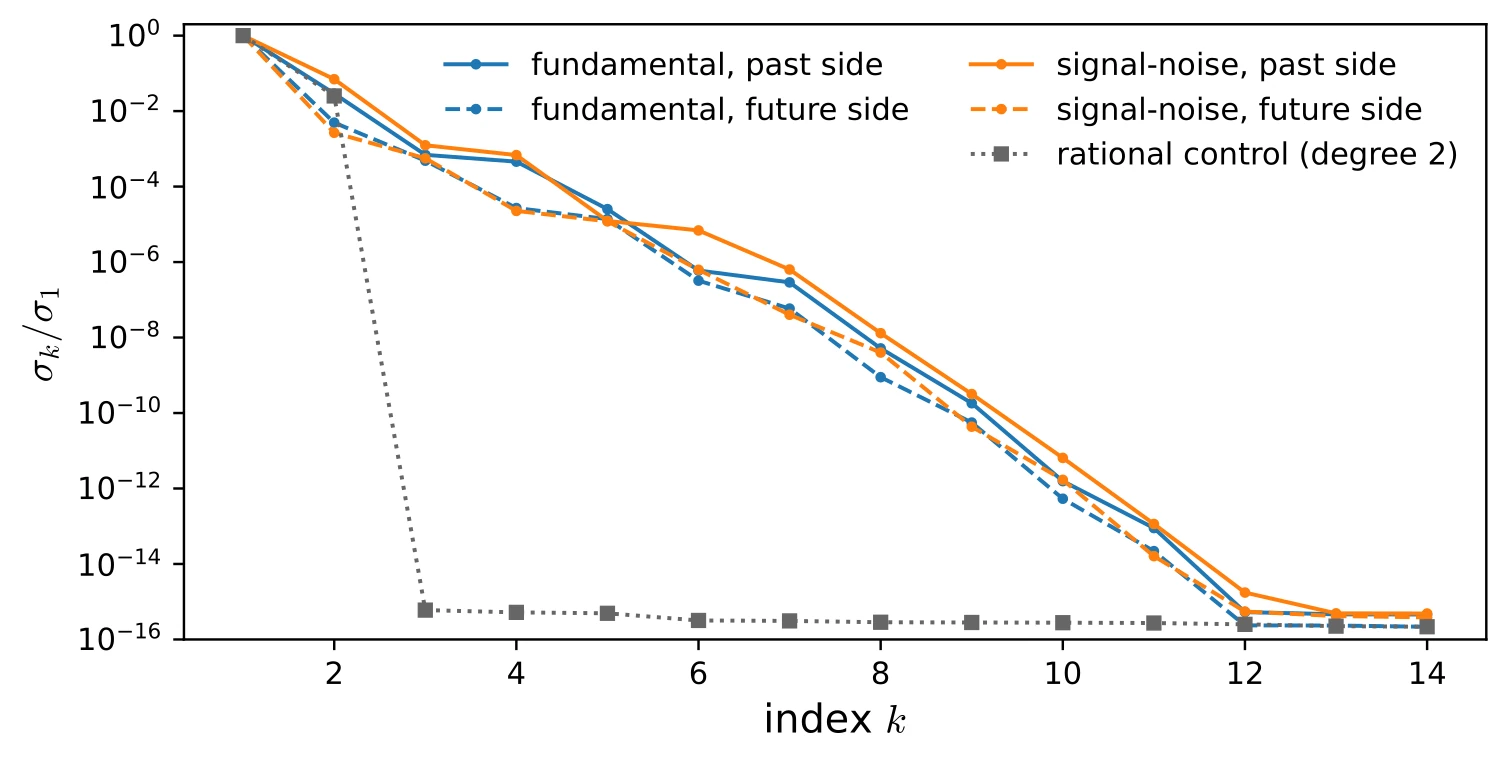
The computed kernels show this. Each one-sided kernel has a sequence of singular values $σ_{1} \geq σ_{2} \geq \dots$ in which $σ_{k + 1}$ is the Hankel-norm error of the best $k$ -dimensional approximation, so a rational kernel of degree $k$ has $σ_{k + 1} = 0$ [1, 44]. Figure 3.4 plots these values for the four one-sided pieces of $h^{X, 1}$ against a rational control of degree two. The control’s third singular value is zero to machine precision. The equilibrium kernels’ singular values fall by a factor of ten to thirty at each index and reach the accuracy of the computation, about $1 0^{- 15}$ , by the twelfth without hitting zero. No low-order Markov state reproduces them exactly. Past the twelfth index the computation cannot distinguish a high degree from an infinite one.

The geometric decay is also a quantitative guarantee. A five-dimensional Markov state reproduces the kernel to better than $1 0^{- 5}$ , and each further dimension gains another factor of ten. No $k$ -dimensional model can do better than $σ_{k + 1}$ , and a truncated belief hierarchy is in general not the optimal $k$ -dimensional approximation, so its error can be much larger than $σ_{k + 1}$ . Recent computational work on asymmetric-information LQG games restricts strategies to a finite-dimensional state from the outset [48, 92, 112]; the singular values lower-bound what any such restriction discards.

Figure 3.4. Singular values $σ_{k}$ of the four one-sided pieces of $h^{X, 1}$ , with an exactly rational kernel of degree two as control.

3.5Conclusion

The stationary system is the finite-horizon noise-state calculus with calendar time removed, and its lag equations give the stationary notation the Kyle–Back chapter uses. Proposition 3.1 verifies that an admissible stationary profile solving these equations is a best response in the noise-state linear class, and the transform identities in Section 3.3 give an alternative representation for solving them. The uniqueness clause needs the Schur complement condition (1.3.3), which fails at zero trading cost, so the Kyle–Back computations run at a small positive cost and Chapter 4 verifies optimality through second-order checks instead. Numerically, the computed kernels cannot be generated by any low-dimensional Markov state, though low-dimensional approximations are accurate (Section 3.4). Whether the infinite-horizon fixed point exists remains open.

3.AComputing the stationary equilibrium

Cutting off lags beyond $L$ and placing them on a grid of fixed spacing turns the filter and adjoint kernels into vectors indexed by age. Delays are shifts of the age index. The kink of $h^{X, i}$ at $ℓ = 0$ reappears at $ℓ = - τ_{k}$ and $ℓ = - Δ_{k}$ , where the delayed kernels are evaluated, and at age $Δ_{i}$ in the filter, so those points are panel boundaries in the spectral scheme.

The natural algorithm alternates between the filtering equations solved forward and the adjoint equations solved backward with damping, and it converges on a coarse grid but fails as the grid is refined. In classical filtering the update is nonexpansive because the observation structure is fixed in advance. Here the observation drift contains the equilibrium kernels themselves, so the projection changes from one iteration to the next. The combined step stops being a contraction as the kink at lag zero becomes steeper on finer grids.

Given the policy kernels, the filtering equations say that the belief loadings are the least-squares projection of each primitive shock onto the observation history. The solver computes that projection directly from the covariance matrix of the observations. That matrix is Toeplitz except in the rows for the shortest ages, and the conjugate gradient method with a circulant preconditioner solves the resulting system [30]. Only the update of the policy kernels remains iterative.

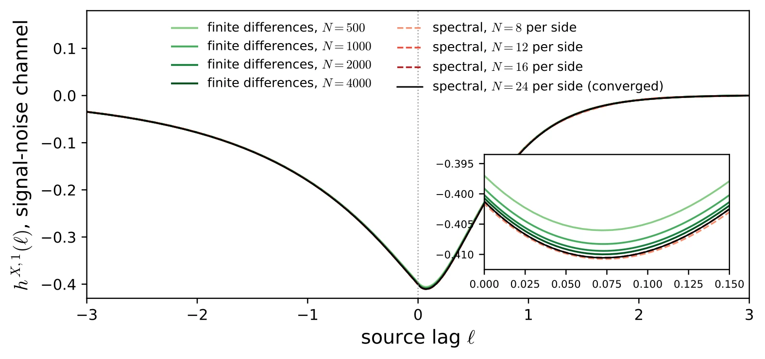
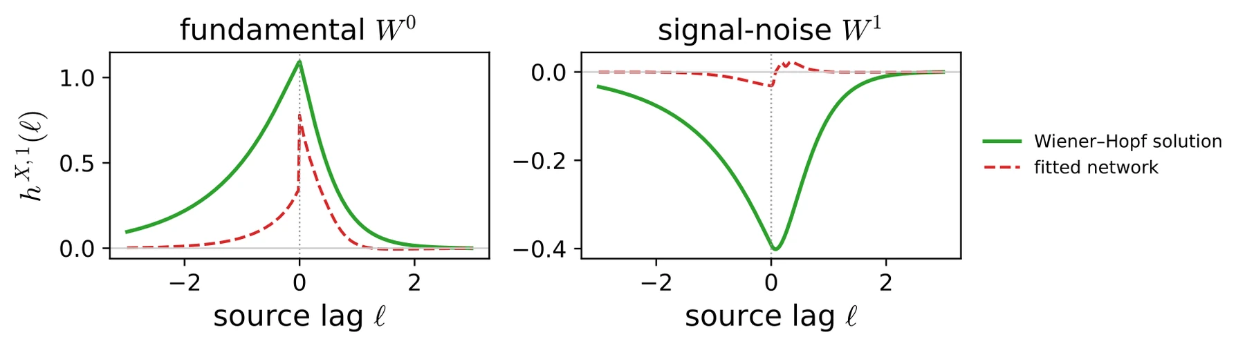
The grid scheme reads the state at the midpoint of each cell, which introduces an error of first order in the spacing. The solutions on grids from $N = 500$ to $N = 4000$ points still move by a few parts in a thousand between refinements. The reported figures therefore come from a second discretization. The kernels are smooth on each side of lag zero, so each one-sided kernel is represented by its values at Chebyshev points on $[0, L]$ , and each two-sided kernel by two such sets on $[- L, 0]$ and $[0, L]$ . The projection, the adjoint transport, and the wedge integrals become small dense matrices built from polynomial interpolation and Gauss–Legendre quadrature, and the equilibrium is found by Newton’s method on the policy values. With 24 points per side the solution is converged to $1 0^{- 13}$ , and a full equilibrium takes about ten milliseconds on a desktop. The grid solutions converge toward it as the spacing shrinks (Figure 3.5), and the depth of the kink agrees with an independent solution by the Wiener–Hopf method [91]. The spectral solution reproduces the closed-form filter of the uncontrolled problem to $3 \times 1 0^{- 8}$ , which is the size of the truncation at $L$ .

Neural networks were also tried. At the fitting points, the networks reduced equation residuals below $2 \times 1 0^{- 3}$ , yet still misrepresented the future-lag side of the fundamental piece and the entire kink at lag zero (Figure 3.6). Small residuals at the fitting points do not show that a network solution is correct, so any such solution should be checked through the finite-deviation identity of Chapter 1.

Figure 3.6. A neural-network solution compared with the Wiener–Hopf solution of the same system, with equation residuals below $2 \times 1 0^{- 3}$ at the fitting points.

The solvers, refinement studies, and figures in this chapter are the work of Claude Fable 5, a large language model built by Anthropic [7], working under the author’s direction. Interactive versions of the dissertation’s computations are collected at sbabichenko.com/noisestate.