Chapter 6Monitored Deviations: Naive Distortions and Privy Responses

6.1Introduction

Chapter 4 retains the classical Kyle–Back division of roles, in which informed traders choose strategic controls while the competitive market maker’s pricing rule is pinned down by conditional-expectation consistency. The price is then not a control the market maker can deviate from unilaterally. A strategic market maker requires a different equilibrium test. Its quote must be an admissible control, and changing the quote unilaterally must not improve its payoff.

Such a deviation is not hidden inside aggregate order flow. In the transparent market, traders observe the information needed to recognize a departure from the market maker’s quote rule. The deviation propagates through the other players’ strategies before returning to the market maker’s objective. Pricing this feedback requires a coordinate for each player who sees the deviation and responds to it, and an adjoint valuing the resulting chain of responses. The finite-horizon response calculus below defines these objects. Applying it to a strategic stationary market maker additionally requires specifying the market maker’s objective, solving the market equilibrium, and translating the gains, one for each pair of a deviating player and a player who responds to it, into the lag coordinates of Chapter 3.

The preceding chapters vary what players know about nature, the projection $W^{i}$ , while every deviation stays hidden inside others’ filtering. This chapter varies what players know about the origin of an off-equilibrium deviation.

In Chapter 1 the deviation’s origin is known exclusively to the deviating player. The deviating player knows the drift it inserted, so its own innovation is invariant, while every other player attributes the resulting movement to primitive shocks and filters it accordingly. The information wedge $V^{i}$ prices this unrecognized-deviation channel. It does not record how another player changes its strategy after recognizing who deviated.

Here a deviation may instead be monitored. A player who knows its origin, a privy player, treats it as a labeled, perfectly observed, zero-variance shock and responds through a separate strategy coordinate. A player who does not know its origin, a naive player, continues to filter its effect as primitive shocks. The same seed can generate privy responses for some players and naive filtering for others. The convention of Chapter 1 is the corner in which no opponent monitors the deviation, while a publicly attributable market-maker quote lies in the opposite corner in which every relevant opponent is privy. When every opponent is privy, a deviation moves no opponent’s beliefs, the information wedge vanishes, and equilibrium play is the separation principle applied to the closed-loop strategies of the perfect-information game [16, 25]. In the classical perfect-information game every player sees the shocks and is privy. The monitoring relation (Definition 6.1) moves the game between these corners; Proposition 6.13 recovers the two endpoints exactly. The naive players here differ from the deceived agents of the adversarial-deception literature [67, 119]. Their strategies remain equilibrium best responses, and their inference is Bayes-correct given their information (Remark 6.3); they lack only the origin label. Table 6.1 locates the four regimes. This chapter mixes the two columns: the same deviation can be observed by some players and unobserved by others.

Table 6.1. Four information regimes. The monitoring relation moves the game along the bottom row, and Proposition 6.13 recovers its two corners exactly; the top row is the classical pair.
	deviations
2-3 shocks	unobserved	observed
observed	open-loop Nash	closed-loop Nash
filtered	Chapter 1	all-privy corner

Mathematically, monitoring enlarges the forward system. A labeled deviation gives every player who sees it a response coordinate, in addition to any shifts in ordinary noise-state estimates, so merely removing privy players from the wedge sum would omit their strategic responses. The response is the linear perturbation implied by the equilibrium policy kernels, not a re-solution of the game after the deviation. For each responder–origin pair one backward equation, (6.5.16), gives a gain $H^{j \leftarrow i}$ , and the response to a seed at any time $t$ is read off by (6.5.23), so no forward–backward system is solved per seed time.

Index roles are fixed throughout this chapter. The pair $j \leftarrow i$ always reads “responder $j$ , origin $i$ .” Symbols carrying $k$ or $k^{'}$ together with $j \leftarrow i$ identify the ordinary noise-state row or column inside that responder–origin map.

6.2Baseline noise-state setting

The objects of Chapter 1 carry over. Let $I = {1, \dots, n}$ be the player set and let the primitive uncertainty be a Brownian shock path $W$ . The state and player $i$ ’s observation evolve as $d X_{t} = (B_{X}^{X} (t) X_{t} + m = 1 \sum n B_{m}^{X} (t) D_{t}^{m}) d t + E^{0} d W_{t}, d Y_{t}^{i} = B_{X}^{Y, i} (t) X_{t} d t + E^{i} d W_{t}, (6.2.1)$ so that player $m$ ’s control enters the state through the control-to-state map $B_{m}^{X}$ , and $B_{X}^{Y, i}$ is the state-to-observation map; $E^{0}$ and $E^{i}$ load the common shocks $W$ into the state and into player $i$ ’s observation. Player $j$ observes a filtration $F_{t}^{j}$ and carries the noise-state $W_{t}^{j} (u) := E [W_{u} ∣ F_{t}^{j}], 0 \leq u \leq t,$ and its equilibrium action is noise-state linear, $D_{t}^{j} = \overset{ˉ}{D}_{t}^{j} + \int_{0}^{t} D_{t}^{j} (u) d W_{t}^{j} (u) . (6.2.3)$ Here “linear” refers to linearity in the represented shock coordinates, not to linearity of the kernels, themselves determined by nonlinear fixed-point equations.

Each player’s running cost is quadratic in the joint physical-state and control variable, as in (1.3.2), with Hessian $G^{j} (s) = (G^{XX, j} (s) G^{D X, j} (s) G^{X D, j} (s) G^{DD, j} (s)), G^{D X, j} (s) = (G^{X D, j} (s))^{⊤} . (6.2.4)$ Throughout, $G^{j} (s)$ satisfies the Schur condition (1.3.3) of Chapter 1.

6.3Deviation origins and monitoring

6.3.1The monitoring relation

The monitoring relation is directed. Every player knows the origin of its own deviation, so the relation is reflexive and the set of privy players includes the deviating player itself. The blip-of-irrationality convention of Section 6.4.2, a single forced departure after which the deviating player resumes equilibrium play, fixes what this means for the deviating player’s own continuation.

Definition 6.1 (Monitoring relation). Write $j ⊵ i$ if player $j$ can resolve deviations whose origin is player $i$ . Equivalently, when player $i$ creates a deviation seed, the impulse that starts the deviation, player $j$ observes its origin perfectly and treats it as a separate deviation shock rather than filtering it as part of the primitive uncertainty. The relation is reflexive, so $i ⊵ i$ for every $i$ . Throughout, a deviation is a control spike $z$ of player $i$ , and $v_{i} = B_{i}^{X} (t) z$ is the state impulse it produces; the seed carried by the forward system is $v_{i}$ , not $z$ . It is the state impulse alone; Chapter 4’s seed was the filter displacement a spike leaves.

For each origin $i$ , define $P_{i} := Privy (i) := {j \in I : j ⊵ i}, N_{i} := Naive (i) := I ∖ P_{i} . (6.3.2)$ The set $P_{i}$ contains every player who observes $i$ ’s deviation seed, the deviating player among them, while $N_{i}$ contains the players who do not.

A common source of the relation is information inclusion. If every information source available to player $i$ is also available to player $j$ (for example $F_{t}^{i} \subseteq F_{t}^{j}$ , with observation of $i$ ’s policy rule and action channel), it is natural to set $j ⊵ i$ . Inclusion is sufficient: $j$ can compute $i$ ’s equilibrium action, and any gap between it and the realized action is $i$ ’s deviation. It is not necessary: $j$ may observe $i$ ’s action directly, a posted quote for instance, without observing $i$ ’s signals, as in Section 6.8. The calculus below requires only the relation $⊵$ ; the modeler specifies the institutional or informational mechanism that generates it.

6.3.2Transitivity

Transitivity is assumed: $k ⊵ j ⊵ i ⟹ k ⊵ i . (6.3.3)$ The condition is substantive. Suppose $j$ is privy to $i$ and so responds to $i$ ’s seed. If $k$ is privy to $j$ but not to $i$ , then $k$ sees $j$ ’s response while lacking the coordinate needed to represent the cause of that response. The response chain is then ill-typed: $k$ can identify the proximate actor but not the root seed, a murder mystery.

Contrapositively, if $k$ is naive to $i$ and $j$ is privy to $i$ , then $k$ must also be naive to $j$ ’s response to $i$ : $k ⋭ i, j ⊵ i ⟹ k ⋭ j for every j responding to the i -seed . (6.3.4)$ Transitivity is the monitoring analogue of partial nestedness in team theory [55]. There, an agent affected by another’s action observes that other’s information; here, a player who sees a response also sees its origin.

Lemma 6.2 (Naive sets). Under transitivity (6.3.3), $N_{i} \subseteq N_{j}$ for every privy player $j \in P_{i}$ . A player naive to the deviating player is naive to every response by a privy player $j \in P_{i}$ . Section 6.5 reads this as a containment of index sets: the rows of every gain, indexed by $N_{j}$ , contain its columns, indexed by $N_{i}$ .

Proof. If $k \in N_{i}$ and $j \in P_{i}$ , then (6.3.4) gives $k ⋭ j$ , so $k \in N_{j}$ . ◻

Remark 6.3 (No smoke without fire). Consider the ill-typed case above, in which $k$ observes player $j$ ’s response to an $i$ -origin seed but not the origin $i$ . Seeing only the response move the state, $k$ could not treat it as a labeled coordinate. It would have to attribute the movement by Bayes’ rule, forming a posterior over which origin produced the response, supported on every deviation $k$ cannot rule out. That posterior is not a free belief but an equilibrium object. Transitivity is exactly the condition that forbids this case. On the privy side the attribution never arises: a privy player’s response kernel $D^{j \leftarrow i}$ is indexed by the originating seed $i$ , not by an inferred mixture over possible origins. To rule out this attribution problem, no player may see smoke without seeing the fire that caused it.

With reflexivity and transitivity, $⊵$ is a preorder. If $i ⊵ j$ and $j ⊵ i$ , then $i$ and $j$ are informed about each other’s deviation origins.

Assumption 6.4 (Perfect transitive monitoring). The relation $⊵$ is reflexive and transitive, and monitoring is perfect: a player either observes a deviation origin exactly or not at all, with no intermediate noisy observation. Formally, $j ⊵ i$ means that player $j$ ’s strategies may depend on the coordinate $z^{i} \in Z_{i}$ of Remark 6.5.

This assumption is maintained for the rest of the chapter; Remark 6.12 returns to the role of perfect observation and to what fails when it is dropped.

6.4Naive versus privy coordinates

Monitoring breaks a convention every other chapter relies on. The control is noise-state linear, (6.2.3), and everything a player could react to reaches it through $W^{j}$ , an opponent’s deviation included, since a deviation enters the observation stream and is filtered like any other movement of the state. A monitored seed is not like that. It moves the physical state, and it moves the beliefs of the players who do not recognize it, but for a player who does recognize it there is nothing to filter. The seed has zero variance under the equilibrium law, so it is not a coordinate of any noise-state, and a strategy written as a function of $W^{j}$ alone cannot respond to it. The response has to live somewhere else. A strategy must therefore split into two parts. The on-path part is the policy kernel of the other chapters. The response part is a kernel on the labeled seed coordinate, zero on the equilibrium path and pinned only by what the player would do off it. Section 6.4.3 makes the decomposed object the strategy of the monitored game.

6.4.1Naive and privy players

A naive player $k \in N_{i}$ does not recognize the deviation seed $v_{i} (s)$ as a deviation. Its physical effect enters $k$ ’s observation stream, and $k$ filters that effect as if it were evidence about the primitive shock path. The ordinary noise-state changes: $δ_{i} w_{t}^{k} (u; s) \neq = 0, k \in N_{i} .$ Throughout, $δ w$ is the noise-state perturbation in density form, $d_{u} δ W_{t}^{k} (u) = δ w_{t}^{k} (u) d u$ ; the singular part $Π^{k} d W_{u}$ does not vary. For a privy player $j \in P_{i}$ , the ordinary shock estimate does not change when $i$ deviates: $δ_{i} w_{t}^{j} (u) = 0 for the ordinary primitive-shock coordinate. (6.4.2)$ Instead, $j$ receives a separate input coordinate, the deviation seed $v_{i} (s)$ (Remark 6.5). The seed enlarges player $j$ ’s sufficient statistic from $W^{j}$ to $(W^{j}, {v_{i} (s) : j ⊵ i}) . (6.4.3)$ This labeled coordinate needs a response kernel of its own.

Remark 6.5 (Deviations on their own factor). Deviations live on their own factor. Let $Z_{i}$ be player $i$ ’s admissible deviations, the $L^{2}$ control paths of Chapter 1, and $Z = \prod_{i} Z_{i}$ . Player $j$ ’s strategy is measurable in $F_{s}^{j}$ and in the factors $Z_{i}$ with $j ⊵ i$ , its own among them, and constant in the others. Under the equilibrium law the seed has zero variance, so a naive player’s filter carries no coordinate for it and never anticipates it; a privy player reads it as a known input. At fixed equilibrium gains the displaced state, filters, and responses are affine in $z \in Z$ , so the coefficients below are exact for finite deviations, and two deviations, from one origin or several, displace by the sum. The seed affects conditional means but not conditional covariances or the ordinary filter for the primitive shocks. A monitored deviation can move a privy player’s action but cannot manipulate that player’s ordinary noise-state. That perfect observation keeps the privy response affine in the seed.

As in the Chapter 1 spike variation, $v$ denotes the induced state impulse, the state movement a control spike produces. The forward variational system starts from $δ_{i} X_{t} = v . (6.4.4)$ If the underlying control-space spike is $z$ , then $v = B_{i}^{X} (t) z$ , and the deviating player’s first-order condition pulls the state price back to control space through $(B_{i}^{X} (t))^{⊤} H_{t}^{X, i}$ . The kernel $D_{t}^{j \leftarrow i} (s)$ represents a privy player’s response per unit of observed state impulse; a control-space spike first maps into the state impulse and then propagates.

6.4.2Blip of irrationality

The convention that fixes how privy players continue off equilibrium is a blip of irrationality, in which a deviation is a single forced departure from $i$ ’s best response, after which $i$ continues through its own response kernel $D^{i \leftarrow i}$ . The other players do not read the blip as evidence about $i$ ’s type or as a loss of reputation. Continuation play treats the deviation as bygone, as in Markov perfect equilibrium [83]. The responders price the mechanical effect of the seed and carry on as though $i$ is again rational.

The seed spawns no independent root seeds. It induces responses that change the state and feed naive filters and other controls, but each response, the deviating player’s own included, is a deterministic linear function of $v_{i} (s)$ within the per-origin system.

Chapter 1 needed no such convention. No opponent observes a deviation’s origin, so how the deviating player’s own future departures are grouped into seeds is invisible to every other player, and only the total control path matters. Once some players are privy, the grouping matters. A responder reacts to each labeled seed it observes, so what counts as one seed with its continuation, rather than several separate seeds, determines the responses. The blip convention pins this down. Given it, the deviating player’s own deviation calculus does not depend on how a departure is decomposed.

Lemma 6.6 (Blip and frozen continuations). Fix an origin $i$ . For a seed time $t$ in the horizon $[0, T]$ of Chapter 1, let $e_{t}$ denote the control spike at $t$ followed by the frozen continuation, as in Corollary 1.11. Let $b_{t}$ denote the same spike followed by the blip continuation, in which $i$ resumes its equilibrium response. Then $b_{t} = e_{t} + \int_{t}^{T} K (s, t) e_{s} d s, (6.4.5)$ where $K$ is the bounded strictly causal kernel generated by the deviating player’s response to its own seed, and $Id + K$ is invertible on the space of admissible $L^{2}$ deviations, the control class of Corollary 1.11. Consequently the families ${e_{t}}$ and ${b_{t}}$ span the same space of admissible deviations, and the deviating player’s first-order condition (6.5.36) is the same under either convention. The deviation quadratic forms of Corollary 1.11, written in the two bases as $Q_{e}$ and $Q_{b}$ , are related by the invertible change of variable $(Id + K)$ , with $Q_{b} = (Id + K)^{*} Q_{e} (Id + K)$ , so one is positive definite (semidefinite) exactly when the other is.

Proof. The two continuations agree on $[0, t]$ and differ on $(t, T]$ by the response path that the blip convention appends, the linear image of the seed under the deviating player’s own response kernels propagated through (6.5.8). This difference is an admissible control path supported on $(t, T]$ , and every such path is a superposition of frozen spikes at times $s > t$ ; reading off the coefficient of $e_{s}$ defines $K (s, t)$ . The kernels are bounded on the compact horizon (admissibility), so $K$ is a bounded Volterra operator and $Id + K$ is invertible. The inverse is given by the series $Id - K + K^{2} - \dots$ , because $K$ is strictly causal, feeding a spike at $t$ only into times after $t$ . Both families parameterize the same space. A linear functional vanishes on a spanning family exactly when it vanishes on the space, which gives the first-order claim. Substituting $b = (Id + K) e$ into the deviation quadratic form gives $Q_{b} = (Id + K)^{*} Q_{e} (Id + K)$ , and an invertible change of variable preserves positive definiteness (semidefiniteness). ◻

The exact finite-deviation identity of Corollary 1.11 transfers through $(Id + K)$ , so verifying a blip-convention profile against all admissible deviations reduces to the Chapter 1 identity.

Monitoring creates two belief freedoms that the all-naive setting of Chapter 1 lacks. A player who sees a movement may need to know who caused it, and a player who sees a seed may need to know what the deviating player will do next. Transitivity closes the first, so no attribution belief is ever needed (Remark 6.3), and the blip convention closes the second by fixing the continuation.

6.4.3The monitored game and its equilibrium

The primitives of the monitored game are the baseline game of Section 6.2, the monitoring preorder of Definition 6.1 under Assumption 6.4, and the blip convention. A strategy for player $j$ has two parts. On the equilibrium path it reduces to the noise-state linear map (6.2.3). Off the path, player $j$ ’s strategy may depend on the coordinates $z^{i}$ with $j ⊵ i$ (Remark 6.5), and it specifies a response kernel pair $(D^{j \leftarrow i, X}, D^{j \leftarrow i, W^{k}})$ for each origin $i$ with $j ⊵ i$ . A player’s full feedback map is the pair of on-path kernels and response kernels.

Definition 6.7 (Monitored-deviation equilibrium). A profile of full feedback maps is a monitored-deviation equilibrium if

for every player $i$ , no admissible control deviation improves $i$ ’s payoff against the other players’ full feedback maps. The deviation’s consequences are generated by the monitoring structure: each privy player responds through its response kernels and each naive player filters the deviation’s effects with its equilibrium filter;
for every origin $i$ , seed, and privy player $j \in P_{i}$ , player $j$ ’s response is optimal for $j$ conditional on the observed seed, against the other players’ full feedback maps.

Condition (ii) is sequential rationality, optimality conditional on events that equilibrium play never produces. A seed occurs with probability zero, so (ii) changes no player’s ex-ante payoff. It pins the response kernels. For $j = i$ it pins the deviating player’s own post-blip continuation. At first order, (ii) is the privy player’s first-order condition (6.5.9), with the response kernels (6.5.23), and (i) is the deviating player’s condition (6.5.36); both come out of the rectangular backward system of Proposition 6.9. Lemma 6.6 lets one verify condition (i) beyond first order. The finite-deviation identity of Corollary 1.11, transported to the blip basis, expresses the payoff change of an arbitrary admissible deviation as its first-order term plus a quadratic form in the deviation. Verification requires this quadratic form to be positive semidefinite.

Existence is a separate question. At the corners, Proposition 6.13 reduces the concept to systems with known existence theory, the coupled Riccati equations of the closed-loop game [16, 26] and the finite-horizon results of Chapter 1. Away from the corners the profile and the response kernels form one fixed-point problem, the one the market of Section 6.8 poses; a general existence theorem is open.

6.5The seed-dependent system

Fix a deviating player $i$ and a seed time $t$ , with privy set $P_{i}$ and naive set $N_{i}$ as in (6.3.2). The state dynamics are (6.2.1), with player $m$ ’s control entering through $B_{m}^{X}$ . We first derive the forward equations and the privy player’s response to the seed. We then write the backward system in operator form and in coefficient blocks, before treating the deviating player’s response to its own seed.

6.5.1Forward deviation equations

The initial condition for a state impulse by player $i$ at time $t$ is $δ_{i} X_{t} = v, δ_{i} w_{t}^{k} (u) = 0 (k \in N_{i}, 0 \leq u \leq t) . (6.5.1)$ For $s \geq t$ , the displaced state is $(δ_{i} X_{s}, {δ_{i} w_{s}^{k} (u) : k \in N_{i}, 0 \leq u \leq s}) .$ The state equation is $\frac{d}{d s} δ_{i} X_{s} = B_{X}^{X} (s) δ_{i} X_{s} + k \in N_{i} \sum \int_{0}^{s} B_{k}^{X} (s) D_{s}^{k} (u) δ_{i} w_{s}^{k} (u) d u + j \in P_{i} \sum B_{j}^{X} (s) δ_{i} D_{s}^{j} . (6.5.3)$ For each naive player $k \in N_{i}$ , define the naive error variation $δ_{i} X_{s}^{k} := δ_{i} X_{s} - \int_{0}^{s} X (s, r) δ_{i} w_{s}^{k} (r) d r . (6.5.4)$ The kernel $X (s, r)$ is the impulse response of the state at $s$ to a primitive shock at $r$ . It carries no player index, since the dynamics are common; integrating it against the truth gives the state, and against a player’s estimates gives that player’s estimate of the state. Player $k$ ’s unresolved-state kernel $X_{s}^{k} (u)$ of Chapter 1 is the part of that response player $k$ has not yet resolved, and its innovation kernel is $C_{s}^{k, Y} (u) := B_{X}^{Y, k} (s) X_{s}^{k} (u) . (6.5.5)$ The naive filter variation has an interior revision equation $\partial_{s} δ_{i} w_{s}^{k} (u) = (C_{s}^{k, Y} (u))^{⊤} B_{X}^{Y, k} (s) δ_{i} X_{s}^{k}, 0 \leq u < s, (6.5.6)$ and a birth term $δ_{i} w_{s}^{k} (s) = E^{k ⊤} B_{X}^{Y, k} (s) δ_{i} X_{s}^{k} . (6.5.7)$ Substituting (6.5.4) into (6.5.6), the coefficient of $δ_{i} w_{s}^{k} (r)$ in $\partial_{s} δ_{i} w_{s}^{k} (u)$ is $- C_{s}^{k, Y} (u)^{⊤} B_{X}^{Y, k} (s) X (s, r) .$ This is the belief–belief block of the generator, and it is not symmetric in $(u, r)$ : the lag $u$ being revised enters through the error kernel, the lag $r$ of the shock being estimated through the state kernel. That asymmetry makes the generator non-self-adjoint.

6.5.2A privy player’s response

Fix a privy player $j \in P_{i}$ . To compute player $j$ ’s response to the origin- $i$ seed, one tests whether $j$ would profitably deviate from its proposed response. This introduces a second, hypothetical, $j$ -origin spike. The $i$ -seed and this test $j$ -seed are distinct labels. In the gain defined below, the rows are indexed by $N_{j}$ , the players naive to $j$ , because they come from player $j$ ’s own deviation problem; the columns by $N_{i}$ , the players naive to $i$ , because they come from the already-realized $i$ -origin displacement.

Let the closed-loop coefficients for an $a$ -origin deviation be $A_{a}^{XX} (s) A_{a}^{X W^{p}} (s, u) := B_{X}^{X} (s) + q \in P_{a} \sum B_{q}^{X} (s) D_{s}^{q \leftarrow a, X}, := B_{p}^{X} (s) D_{s}^{p} (u) + q \in P_{a} \sum B_{q}^{X} (s) D_{s}^{q \leftarrow a, W^{p}} (u), p \in N_{a} . (6.5.8)$ These coefficients use the response kernels appropriate to the origin label $a$ . When $a = i$ they propagate the observed $i$ -seed; when $a = j$ they are the row-side coefficients that price a hypothetical deviation by $j$ .

The $i$ -variation of player $j$ ’s closed-loop adjoint has rows $δ_{i} H_{s}^{X, j}$ and $δ_{i} H_{s}^{W^{k^{'}}, j} (u)$ for $k^{'} \in N_{j}$ , dual to the row state $S^{j}$ of (6.5.11). The next two subsections write it as one rectangular gain, first in operator form and then in coefficient blocks, with source $G_{eff}^{j \leftarrow i}$ .

Player $j$ ’s first-order condition, conditioned on its own information $F_{s}^{j}$ , gives its response. Player $j$ ’s strategies are measurable in the factor $Z_{i}$ (Remark 6.5), so the origin- $i$ seed is a known input to $j$ . Subtracting the condition player $j$ satisfies on the equilibrium path from the one it satisfies after the $i$ -seed gives $0 = G^{DD, j} (s) δ_{i} D_{s}^{j} + G^{D X, j} (s) δ_{i} X_{s} + E [(B_{j}^{X} (s))^{⊤} δ_{i} H_{s}^{X, j} ∣ F_{s}^{j}] . (6.5.9)$ Player $j$ observes the $i$ -seed, and the forward and adjoint systems are linear with deterministic coefficients, so the conditional expectation collapses: $δ_{i} D_{s}^{j} = - (G^{DD, j} (s))^{- 1} [G^{D X, j} (s) δ_{i} X_{s} + (B_{j}^{X} (s))^{⊤} δ_{i} H_{s}^{X, j}] . (6.5.10)$

Remark 6.8 (Two labels, no cross term). The forward system is affine in the seeds, so the $i$ - and $j$ -labeled forward effects add, and the test uses the same gains as the ordinary $j$ -origin deviation problem. The $i$ -seed shifts the value of player $j$ ’s adjoint while leaving that gain system intact.

6.5.3Operator form and source

The operator notation compresses the seed-dependent physical and noise-state equations above. Stacked symbols collect Chapter 1 coordinates, and the rectangular gain $H^{j \leftarrow i}$ collects their adjoint responses into one backward solve.

An $i$ -origin seed moves the noise-states of $N_{i}$ , while a hypothetical deviation by $j$ moves those of $N_{j}$ . There is then no single displaced state, so the origin label indexes the state. For any origin label $a$ , define the state attached to that origin by $S_{s}^{a} := (X_{s}, {W_{s}^{p} (u) : p \in N_{a}, 0 \leq u < s}) . (6.5.11)$ The superscript $a$ is the origin label, and the noise-state fields are those of the players naive to origin $a$ .

For an $a$ -origin deviation, write $δ_{a} S_{s}^{a} := (δ_{a} X_{s}, {δ_{a} w_{s}^{p} (u) : p \in N_{a}}) . (6.5.12)$ The deviation dynamics are $\frac{d}{d s} δ_{a} S_{s}^{a} = A_{a} (s) δ_{a} S_{s}^{a}, A_{a} (s) = A_{a}^{tr} (s) + A_{a}^{fil} (s), (6.5.13)$ where $A_{a}^{tr}$ is the controlled-state transport part and $A_{a}^{fil}$ is the filter birth-and-revision part. Throughout, $A_{a}$ is the full generator and $A_{a}^{XX}$ its physical-state block.

In coordinates, the $X$ row is (6.5.3) with the coefficients (6.5.8) at label $a$ , and the filter rows are (6.5.6)–(6.5.7) for $p \in N_{a}$ . The same non-self-adjoint generator template is used for every origin label. On the row side of a Sylvester equation it is $A_{a}^{*}$ ; on the column side, $A_{a}$ .

Fix an observed seed of origin $i$ and a privy player $j \in P_{i}$ . The $i$ -origin state $S^{i}$ supplies the columns and $S^{j}$ the rows, because player $j$ ’s adjoint lies in the dual of $S^{j}$ . The rectangular gain is then one operator $H_{s}^{j \leftarrow i} : S_{s}^{i} ⟶ (S_{s}^{j})^{*}, δ_{i} H_{s}^{S^{j}} = H_{s}^{j \leftarrow i} δ_{i} S_{s}^{i} . (6.5.14)$ In block form, $H_{s}^{j \leftarrow i} = (H_{s}^{XX, j \leftarrow i} {H_{s}^{W^{k^{'}} X, j \leftarrow i} (u)}_{k^{'} \in N_{j}} {H_{s}^{X W^{k}, j \leftarrow i} (r)}_{k \in N_{i}} {H_{s}^{W^{k^{'}} W^{k}, j \leftarrow i} (u, r)}_{k^{'} \in N_{j}, k \in N_{i}}) . (6.5.15)$

At the operator level, the backward equation is the rectangular Sylvester equation $- \frac{d}{d s} H_{s}^{j \leftarrow i} = G_{eff, s}^{j \leftarrow i} + A_{j} (s)^{*} H_{s}^{j \leftarrow i} + H_{s}^{j \leftarrow i} A_{i} (s), H_{T}^{j \leftarrow i} = Π_{X}^{j, ⊤} G^{XX, j} (T) Π_{X}^{i} . (6.5.16)$

The source is player $j$ ’s ordinary running cost, differentiated once along $j$ ’s own deviation direction and once along the $i$ -seed direction, the Hessian $G^{j}$ evaluated on the two directions. Let $Π_{X}^{a} : S^{a} \to X$ be the physical-state projection. Let $D^{j \leftarrow j} : S^{j} \to D^{j}$ be player $j$ ’s response to its own seed, and let $D^{j \leftarrow i} : S^{i} \to D^{j}$ be player $j$ ’s response to an $i$ -origin seed. Then $G_{eff, s}^{j \leftarrow i} = (Π_{X}^{j} D^{j \leftarrow j})^{⊤} G^{j} (s) (Π_{X}^{i} D^{j \leftarrow i}) . (6.5.17)$ For $j = i$ , the row and column maps coincide and $G_{eff}^{i \leftarrow i}$ is symmetric. For $j \neq = i$ , $G_{eff}^{j \leftarrow i}$ is generally rectangular and nonsymmetric.

Write the response kernels as $δ_{i} D_{s}^{j} δ_{j} D_{s}^{j} = D_{s}^{j \leftarrow i, X} δ_{i} X_{s} + k \in N_{i} \sum \int_{0}^{s} D_{s}^{j \leftarrow i, W^{k}} (r) δ_{i} w_{s}^{k} (r) d r, = D_{s}^{j \leftarrow j, X} δ_{j} X_{s} + k^{'} \in N_{j} \sum \int_{0}^{s} D_{s}^{j \leftarrow j, W^{k^{'}}} (u) δ_{j} w_{s}^{k^{'}} (u) d u . (6.5.18)$ Then the source blocks of (6.5.17) are $G_{eff, s}^{XX, j \leftarrow i} G_{eff, s}^{X W^{k}, j \leftarrow i} (r) G_{eff, s}^{W^{k^{'}} X, j \leftarrow i} (u) G_{eff, s}^{W^{k^{'}} W^{k}, j \leftarrow i} (u, r) = G^{XX, j} (s) + G^{X D, j} (s) D_{s}^{j \leftarrow i, X} + (D_{s}^{j \leftarrow j, X})^{⊤} G^{D X, j} (s) + (D_{s}^{j \leftarrow j, X})^{⊤} G^{DD, j} (s) D_{s}^{j \leftarrow i, X}, = G^{X D, j} (s) D_{s}^{j \leftarrow i, W^{k}} (r) + (D_{s}^{j \leftarrow j, X})^{⊤} G^{DD, j} (s) D_{s}^{j \leftarrow i, W^{k}} (r), = (D_{s}^{j \leftarrow j, W^{k^{'}}} (u))^{⊤} G^{D X, j} (s) + (D_{s}^{j \leftarrow j, W^{k^{'}}} (u))^{⊤} G^{DD, j} (s) D_{s}^{j \leftarrow i, X}, = (D_{s}^{j \leftarrow j, W^{k^{'}}} (u))^{⊤} G^{DD, j} (s) D_{s}^{j \leftarrow i, W^{k}} (r) . (6.5.19) (6.5.20) (6.5.21) (6.5.22)$

The response kernels themselves are $D_{s}^{j \leftarrow i, X} D_{s}^{j \leftarrow i, W^{k}} (r) := - (G^{DD, j} (s))^{- 1} [G^{D X, j} (s) + (B_{j}^{X} (s))^{⊤} H_{s}^{XX, j \leftarrow i}], := - (G^{DD, j} (s))^{- 1} (B_{j}^{X} (s))^{⊤} H_{s}^{X W^{k}, j \leftarrow i} (r), k \in N_{i} . (6.5.23)$ Together, (6.5.16), (6.5.17), and (6.5.23) form a rectangular Riccati–Sylvester fixed point.

6.5.4Coefficient blocks

The gain equations are the coefficient form of the seed-dependent system. The four block equations below share one backward template, specialized to a row coefficient and a column coefficient.

Proposition 6.9 (Rectangular gain reduction). Fix an origin $i$ and a privy player $j \in P_{i}$ . Under Assumption 6.4, suppose the variations $δ_{i} H^{X, j}$ and $δ_{i} H^{W^{k^{'}}, j}$ , $k^{'} \in N_{j}$ , are linear in $(δ_{i} X, δ_{i} w^{k})$ with bounded deterministic coefficients. Then they take the rectangular form $δ_{i} H_{s}^{X, j} = H_{s}^{XX, j \leftarrow i} δ_{i} X_{s} + k \in N_{i} \sum \int_{0}^{s} H_{s}^{X W^{k}, j \leftarrow i} (r) δ_{i} w_{s}^{k} (r) d r, (6.5.24)$ $δ_{i} H_{s}^{W^{k^{'}}, j} (u) = H_{s}^{W^{k^{'}} X, j \leftarrow i} (u) δ_{i} X_{s} + k \in N_{i} \sum \int_{0}^{s} H_{s}^{W^{k^{'}} W^{k}, j \leftarrow i} (u, r) δ_{i} w_{s}^{k} (r) d r . (6.5.25)$ The coefficient functions solve (6.5.28)–(6.5.32), with source blocks (6.5.19)–(6.5.22). Equation (6.5.23) then recovers player $j$ ’s response to any realized origin- $i$ seed without solving a new forward-backward system for each seed time.

The filter contraction.

The filter generator enters the adjoint through one operator and its transpose. For a naive player $k^{'}$ , the filter contraction of Chapter 1, equation (1.4.9), acts here on a noise-state lag field $M$ by $B^{k^{'}} M := E^{k^{'}} M (s) + \int_{0}^{s} C_{s}^{k^{'}, Y} (r) M (r) d r, (6.5.26)$ the filter birth $E^{k^{'}}$ at lag $s$ together with the revision $C^{k^{'}, Y}$ at interior lags. Its transpose acts on a field $N$ from the right, $N B^{k^{'} ⊤} := N (s) E^{k^{'} ⊤} + \int_{0}^{s} N (r) (C_{s}^{k^{'}, Y} (r))^{⊤} d r . (6.5.27)$ Contracting the responder’s $W^{k^{'}}$ -row on the left, $B^{k^{'}} H_{s}^{W^{k^{'}} \cdot}$ for $k^{'} \in N_{j}$ , gives the cost to player $j$ of having its own hypothetical deviation treated as noise by the players naive to it, the sum over $N_{j}$ in (6.5.28). Contracting the deviating player’s $W^{k}$ -column on the right, $H_{s}^{\cdot W^{k}} B^{k ⊤}$ for $k \in N_{i}$ , gives the term through which the deviating player’s seed enters the naive filters, the sum over $N_{i}$ there. Each contraction leaves the other lag as the displayed argument. The observation map $B_{X}^{Y, k} (s)$ multiplies the column contraction on the right in the gain equations below.

Figure 6.1 assembles the four equations as a block. The state $X$ and the naive coordinates $W^{k^{'}}$ ( $k^{'} \in N_{j}$ ) and $W^{k}$ ( $k \in N_{i}$ ) index the rows and columns, and $B_{a} := B_{X}^{Y, a} (s)$ .

Figure 6.1. Reconstructing the backward system $- \dot{H}^{∙∙} = G_{eff}^{∙∙} + A_{j}^{*} H + H A_{i}$ . Row terms come from $A_{j}^{*} H$ (left), column terms from $H A_{i}$ (top); the $W^{k^{'}}$ -row revision and the $W^{k}$ -column residual term carry the opposite sign. Each cell is completed by adding the two terms on its row margin and the two on its column margin; the dot is the free index, filled by the cell’s column on the row margins and by its row on the column margins.

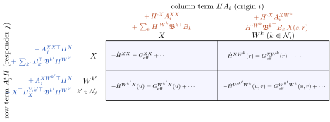
Rows.

Matching the $δ_{i} X_{s}$ coefficient gives $- \frac{d}{d s} H_{s}^{XX, j \leftarrow i} = G_{eff, s}^{XX, j \leftarrow i} + A_{j}^{XX} (s)^{⊤} H_{s}^{XX, j \leftarrow i} + H_{s}^{XX, j \leftarrow i} A_{i}^{XX} (s) + k^{'} \in N_{j} \sum B_{X}^{Y, k^{'}} (s)^{⊤} B^{k^{'}} H_{s}^{W^{k^{'}} X, j \leftarrow i} + k \in N_{i} \sum H_{s}^{X W^{k}, j \leftarrow i} B^{k ⊤} B_{X}^{Y, k} (s), H_{T}^{XX, j \leftarrow i} = G^{XX, j} (T) . (6.5.28)$ Here and below the terminal condition appears blockwise; all non- $XX$ terminal blocks are zero, matching the operator terminal $Π_{X}^{j, ⊤} G^{XX, j} (T) Π_{X}^{i}$ of (6.5.16).

For each $k \in N_{i}$ , matching the coefficient of $δ_{i} w_{s}^{k} (r)$ gives $- \frac{d}{d s} H_{s}^{X W^{k}, j \leftarrow i} (r) = G_{eff, s}^{X W^{k}, j \leftarrow i} (r) + A_{j}^{XX} (s)^{⊤} H_{s}^{X W^{k}, j \leftarrow i} (r) + H_{s}^{XX, j \leftarrow i} A_{i}^{X W^{k}} (s, r) - H_{s}^{X W^{k}, j \leftarrow i} B^{k ⊤} B_{X}^{Y, k} (s) X (s, r) + k^{'} \in N_{j} \sum B_{X}^{Y, k^{'}} (s)^{⊤} B^{k^{'}} H_{s}^{W^{k^{'}} W^{k}, j \leftarrow i} (r), H_{T}^{X W^{k}, j \leftarrow i} (r) = 0. (6.5.29)$ The $X (s, r)$ term inherits its sign from the residual convention $δ_{i} X_{s}^{k} = δ_{i} X_{s} - \int_{0}^{s} X (s, r) δ_{i} w_{s}^{k} (r) d r .$ For each row $k^{'} \in N_{j}$ , matching the $δ_{i} X_{s}$ coefficient gives $- \frac{d}{d s} H_{s}^{W^{k^{'}} X, j \leftarrow i} (u) = G_{eff, s}^{W^{k^{'}} X, j \leftarrow i} (u) + A_{j}^{X W^{k^{'}}} (s, u)^{⊤} H_{s}^{XX, j \leftarrow i} - X (s, u)^{⊤} B_{X}^{Y, k^{'}} (s)^{⊤} B^{k^{'}} H_{s}^{W^{k^{'}} X, j \leftarrow i} + H_{s}^{W^{k^{'}} X, j \leftarrow i} (u) A_{i}^{XX} (s) + k \in N_{i} \sum H_{s}^{W^{k^{'}} W^{k}, j \leftarrow i} (u) B^{k ⊤} B_{X}^{Y, k} (s), H_{T}^{W^{k^{'}} X, j \leftarrow i} (u) = 0. (6.5.31)$ For each row $k^{'} \in N_{j}$ and column $k \in N_{i}$ , matching the coefficient of $δ_{i} w_{s}^{k} (r)$ gives $- \frac{d}{d s} H_{s}^{W^{k^{'}} W^{k}, j \leftarrow i} (u, r) = G_{eff, s}^{W^{k^{'}} W^{k}, j \leftarrow i} (u, r) + A_{j}^{X W^{k^{'}}} (s, u)^{⊤} H_{s}^{X W^{k}, j \leftarrow i} (r) - X (s, u)^{⊤} B_{X}^{Y, k^{'}} (s)^{⊤} B^{k^{'}} H_{s}^{W^{k^{'}} W^{k}, j \leftarrow i} (r) + H_{s}^{W^{k^{'}} X, j \leftarrow i} (u) A_{i}^{X W^{k}} (s, r) - H_{s}^{W^{k^{'}} W^{k}, j \leftarrow i} (u) B^{k ⊤} B_{X}^{Y, k} (s) X (s, r), H_{T}^{W^{k^{'}} W^{k}, j \leftarrow i} (u, r) = 0. (6.5.32)$ Together these are the rectangular backward system. It is nonlinear because the response kernels in (6.5.23) and the source blocks (6.5.19)–(6.5.22) depend algebraically on the same coefficients.

6.5.5The deviating player’s own response and its first-order condition

By reflexivity, the deviating player is one of the privy players. Under the blip-of-irrationality convention (Section 6.4.2), the deviating player’s post-blip continuation is its equilibrium continuation law, so its response to its own seed is the diagonal response $D^{i \leftarrow i}$ . The diagonal $j = i$ solves a backward equation of the form $\dot{H}^{i \leftarrow i} = - G_{eff}^{i \leftarrow i} - A_{i}^{*} H^{i \leftarrow i} - H^{i \leftarrow i} A_{i}$ , a source plus the generator acting on each side. It is the rectangular Sylvester equation (6.5.16) at $j = i$ , expanded into the blocks (6.5.28)–(6.5.32). It is special in two ways. First, the deviating player’s continuation control moves with the seed, so its own response is charged in the second variation rather than dropped. Second, the row and column maps coincide. The source is $i$ ’s running-cost Hessian evaluated on its own response kernel, $G_{eff, s}^{i \leftarrow i} = (Π_{X}^{i} D^{i \leftarrow i})^{⊤} G^{i} (s) (Π_{X}^{i} D^{i \leftarrow i}) . (6.5.33)$ Here $Π_{X}^{i}$ is the physical-state projection of (6.5.17). Contracting the $j = i$ case of (6.5.19)–(6.5.22) against the seed gives, on the $X$ row, $[G_{eff, s}^{i \leftarrow i} δ_{i} S_{s}^{i}]^{X} = G_{eff, s}^{XX, i \leftarrow i} δ_{i} X_{s} + k \in N_{i} \sum \int_{0}^{s} G_{eff, s}^{X W^{k}, i \leftarrow i} (r) δ_{i} w_{s}^{k} (r) d r, (6.5.34)$ and, on each belief row, $[G_{eff, s}^{i \leftarrow i} δ_{i} S_{s}^{i}]^{W^{k}} (u) = G_{eff, s}^{W^{k} X, i \leftarrow i} (u) δ_{i} X_{s} + k^{'} \in N_{i} \sum \int_{0}^{s} G_{eff, s}^{W^{k} W^{k^{'}}, i \leftarrow i} (u, r) δ_{i} w_{s}^{k^{'}} (r) d r . (6.5.35)$

The deviating player’s first-order condition sets to zero the coefficient of an arbitrary $F_{t}^{i}$ -measurable control spike: $0 = E [G_{t}^{DD, i} D_{t}^{i} + G_{t}^{D X, i} X_{t} + (B_{i}^{X} (t))^{⊤} H_{t}^{X, i} ∣ F_{t}^{i}], (6.5.36)$ or equivalently $D_{t}^{i} = - (G_{t}^{DD, i})^{- 1} E [G_{t}^{D X, i} X_{t} + (B_{i}^{X} (t))^{⊤} H_{t}^{X, i} ∣ F_{t}^{i}] . (6.5.37)$ Read as a response kernel rather than a level, this condition is the $j = i$ case of (6.5.10).

Remark 6.10 (Symmetry of the own-response equation without a self-adjoint generator). The diagonal equation has the form $\dot{H}^{i \leftarrow i} = - G_{eff}^{i \leftarrow i} - A_{i}^{*} H^{i \leftarrow i} - H^{i \leftarrow i} A_{i} .$ The full generator $A_{i}$ is not self-adjoint, by the belief–belief asymmetry noted after (6.5.6), so the row and column equations need not look term-by-term symmetric. What is symmetric is the diagonal source and terminal condition, so the solution preserves the adjoint symmetry $H^{X W^{k}, i \leftarrow i} (r) = (H^{W^{k} X, i \leftarrow i} (r))^{⊤}, H^{W^{k^{'}} W^{k}, i \leftarrow i} (u, r) = (H^{W^{k} W^{k^{'}}, i \leftarrow i} (r, u))^{⊤},$ provided the backward system has a unique solution.

6.6Superposition under perfect monitoring

For a fixed origin $i$ , the privy players in $P_{i}$ all see the same seed and solve one self-consistency problem, coupled only through the shared forward state. The monitoring relation orders who sees whose seeds. Each origin produces its own gain system of the form (6.5.28)–(6.5.32); the systems differ because the naive/privy split depends on the origin.

Write $R_{t}^{\leftarrow i} (s)$ for the per-unit privy response to an origin- $i$ seed at time $s$ , and $R_{t}$ for the response to a configuration of seeds.

Proposition 6.11 (Superposition of monitored seeds). Under Assumption 6.4, the forward system is affine in the seeds, so the response to several monitored seeds is the sum of the single-seed responses, $R_{t} (m \sum v_{i_{m}} (s_{m})) = m \sum R_{t}^{\leftarrow i_{m}} (s_{m}) v_{i_{m}} (s_{m}) . (6.6.1)$

If player $i$ blips, then the response is the same regardless of whether some other player $j$ blipped sooner or not. Without superposition, verifying would mean thinking about an infinite tree of deviations rather than treating them one at a time. The gains themselves are solved in order rather than independently, since the source (6.5.19) for $j \neq = i$ contains $D^{j \leftarrow j}$ , player $j$ ’s response to its own seed, so each $j \leftarrow i$ solve uses the $j \leftarrow j$ solve first. The pairs $j \leftarrow i$ with $j \neq = i$ for one origin are coupled through $A_{i}^{XX}$ , which contains every $D^{q \leftarrow i, X}$ , $q \in P_{i}$ .

Remark 6.12 (The role of perfect observation). The linear theory relies on binary monitoring. A player either observes a deviation seed perfectly, as a known zero-variance input not jointly estimated with the fundamentals, or not at all, in which case it is folded into the ordinary filter with the equilibrium filter fixed. Keep two relaxations apart. In the first, a player observes the seed through an additive noisy channel. A noisy reading of a point mass at zero carries no information, so this channel is informative only if the seed carries a nondegenerate prior. Deviations then occur with positive probability on the equilibrium path, and the object being solved is no longer a deviation calculus. In the second, transitivity fails and a player sees a response whose origin it cannot resolve. The response discrepancy is identically zero on the equilibrium path, so the observation is a null event, and attribution conditional on it is a mixture over the origins the player cannot rule out. The mixture weights play the role that off-path beliefs play in sequential equilibrium [68]. Given the weights the theory remains linear, but superposition fails, since attribution couples the per-origin blocks into one system.

6.7The two corners

For a fixed origin $i$ , solve (6.5.28)–(6.5.32) for each privy player $j \in P_{i}$ . By Lemma 6.2 the columns $N_{i}$ are contained in the rows $N_{j}$ .

The variations $δ_{i} H^{X, j}$ and $δ_{i} H^{W^{k^{'}}, j}$ in (6.5.24)–(6.5.25) are the marginal values of the seed to player $j$ . The responder’s own first-order condition pins each response kernel; none is assumed. This is the consistency required of conjectured reactions in oligopoly theory [22], and the selection that closed-loop differential games otherwise leave open [16].

The two corners of the monitoring relation recover the two classical regimes.

Proposition 6.13 (Corner reductions). Maintain Assumption 6.4. (i) (All privy.) Fix an origin $i$ with $N_{i} = \emptyset$ . Then the diagonal $j = i$ of (6.5.28)–(6.5.32) retains only its $XX$ block, a Riccati equation in $H^{XX, i \leftarrow i}$ with row and column coefficient $A_{i}^{XX}$ . If $P_{a} = I$ for every origin $a$ , so every naive set is empty, then every solve retains only its $XX$ block and its solution does not depend on the origin, $H_{s}^{XX, j \leftarrow i} = H_{s}^{XX, j}$ for all $i$ . Writing $D_{s}^{j, X}$ for the common response kernel $D_{s}^{j \leftarrow i, X}$ , the pairs $(H^{XX, j}, D^{j, X})$ solve the coupled Riccati system of the closed-loop Nash equilibrium of the perfect-information game [16, 26], $- \dot{H}_{s}^{XX, j} D_{s}^{j, X} A^{XX} (s) = G^{XX, j} (s) + G^{X D, j} (s) D_{s}^{j, X} + (D_{s}^{j, X})^{⊤} G^{D X, j} (s) + (D_{s}^{j, X})^{⊤} G^{DD, j} (s) D_{s}^{j, X} + A^{XX} (s)^{⊤} H_{s}^{XX, j} + H_{s}^{XX, j} A^{XX} (s), H_{T}^{XX, j} = G^{XX, j} (T), = - (G^{DD, j} (s))^{- 1} [G^{D X, j} (s) + (B_{j}^{X} (s))^{⊤} H_{s}^{XX, j}], = B_{X}^{X} (s) + m \sum B_{m}^{X} (s) D_{s}^{m, X} . (6.7.1)$ No seed moves any player’s ordinary filter. (ii) (All naive.) Fix an origin $i$ with $P_{i} = {i}$ . Then only the diagonal $j = i$ remains, and its rows and columns are both indexed by $N_{i} = I ∖ {i}$ . The system (6.5.28)–(6.5.32) is the coefficient form of the $i$ -variation of the adjoint system of Theorem 1.8 of Chapter 1, written in the blip basis of Lemma 6.6, and the exact verification identity of Corollary 1.11 transfers through the basis map.

Proof. (i) With $N_{i} = \emptyset$ the diagonal has no rows or columns beyond $X$ , so only (6.5.28) remains, its source the $j = i$ case of (6.5.19) and its row and column coefficient $A_{i}^{XX}$ . With every naive set empty the $W$ rows and columns are absent for every pair. The candidate $H^{XX, j \leftarrow i} = H^{XX, j}$ matches the terminal condition for every pair. Substituting it into (6.5.23) gives $D^{j \leftarrow i, X} = D^{j, X}$ independent of the origin, so $A_{a}^{XX} = A^{XX}$ for every origin label $a$ in (6.5.8), and the source (6.5.19) becomes the first four terms of (6.7.1). The right sides of (6.5.28) and (6.7.1) then coincide, so the candidate solves the corner system, and it is the solution whenever the closed-loop Riccati system (6.7.1) has a unique solution. That no seed moves any ordinary filter is (6.4.2) applied to every player.

(ii) With $P_{i} = {i}$ only the diagonal pair remains, with rows and columns both indexed by the deviating player’s naive set. Expanding the $i$ -variation of (1.4.7)–(1.4.8) of Chapter 1 in the coefficients of $(δ_{i} X, δ_{i} w^{k})$ and comparing with (6.5.28)–(6.5.32), the terms of (6.5.19) in $D^{i \leftarrow i}$ and the closed-loop part of the row and column coefficient $A_{i}^{XX}$ differ from the frozen-continuation expansion by $G^{X D, i} D_{s}^{i \leftarrow i, X} + (D_{s}^{i \leftarrow i, X})^{⊤} G^{D X, i} + (D_{s}^{i \leftarrow i, X})^{⊤} G^{DD, i} D_{s}^{i \leftarrow i, X} + H_{s}^{XX, i \leftarrow i} B_{i}^{X} D_{s}^{i \leftarrow i, X} + (D_{s}^{i \leftarrow i, X})^{⊤} (B_{i}^{X})^{⊤} H_{s}^{XX, i \leftarrow i} = - (D_{s}^{i \leftarrow i, X})^{⊤} G^{DD, i} D_{s}^{i \leftarrow i, X},$ by the $j = i$ case of (6.5.23) and its transpose, and blockwise the same for the $W$ rows and columns, so the two systems differ by the operator $- (D^{i \leftarrow i})^{*} G^{DD, i} D^{i \leftarrow i}$ . The two conventions are the two continuations of Lemma 6.6, whose change of variable $Q_{b} = (Id + K)^{*} Q_{e} (Id + K)$ carries this term, and the lemma transfers the verification identity. ◻

Remark 6.14 (Lyapunov and Riccati forms). The frozen continuation holds the deviating player’s control fixed after the spike, so its backward equation is linear in $H$ , a Lyapunov equation. The blip continuation lets the deviating player re-optimize, and substituting the gain (6.5.23) makes the equation quadratic in $H$ , a Riccati equation. The term $- (D^{i \leftarrow i, X})^{⊤} G^{DD, i} D^{i \leftarrow i, X}$ is the value of that re-optimization.

6.8A strategic market maker: transparent and opaque markets

In the Kyle–Back markets of Chapter 4 the market maker is not a player. It posts the conditional expectation of the fundamental given order flow, and the only strategic question is how the informed traders trade against that rule. Here the market maker chooses its quote and cares about its inventory, and whether the trader can see its deviations depends on whether order flow is published. Publishing the flow turns the same market, with the same information on the equilibrium path, from a naive corner into a privy one. The market maker observes the order flow, so its observation loads on the trader’s control rather than on the state, which puts the market outside the baseline (6.2.1) and inside Chapter 4. The origin sets and the blip convention are those of this chapter; the trader’s response kernels come from Chapter 4’s adjoint system.

6.8.1The market

One asset, one informed trader (player $1$ ), one market maker (player $0$ ), a finite horizon $T$ . The fundamental $V_{t}$ is a Brownian motion with variance rate $Σ_{V}$ , the market maker posts a quote $P_{t}$ , and both players’ payoffs depend on the two only through the mispricing $M_{t} := V_{t} - P_{t}, (6.8.1)$ the gap between what the asset is worth and what it is quoted at. The trader observes the signal flow $d Y_{t} = M_{t} d t + d W_{t}^{Y}$ of Chapter 4 and submits an order rate $D_{t}$ ; noise traders submit $Σ_{Z}^{1/2} d W_{t}^{Z}$ ; the market maker sees the total order flow $d Z_{t} = D_{t} d t + Σ_{Z}^{1/2} d W_{t}^{Z}$ and absorbs it into its inventory, $d Q_{t} = - d Z_{t} . (6.8.4)$ The trader is risk neutral with a quadratic trading cost and earns the mispricing on its orders, $E \int_{0}^{T} [M_{t} D_{t} - ϵ D_{t}^{2}] d t,$ and the market maker pays it on the flow it absorbs and pays for inventory, $E \int_{0}^{T} [- M_{t} D_{t} - γ Q_{t}^{2}] d t, γ > 0. (6.8.6)$ The mispricing is both the market maker’s control and something it does not know. It sets $M_{t}$ through its quote, but only up to its own estimation error: with $V_{t}^{0} = E [V_{t} ∣ F_{t}^{0}]$ , $M_{t} = M_{t}^{0} + (V_{t} - V_{t}^{0}), M_{t}^{0} := E [M_{t} ∣ F_{t}^{0}] = V_{t}^{0} - P_{t}, (6.8.7)$ and $M_{t}^{0}$ is its control; $M_{t}^{0} > 0$ is a quote below the belief. The trader likewise acts on its own estimate $M_{t}^{1} := E [M_{t} ∣ F_{t}^{1}] = V_{t}^{1} - P_{t}$ , which for the trader is a state of its filter. The state is $(M_{t}, Q_{t})$ , of which only $Q_{t}$ has dynamics of its own; the shocks are $(W^{V}, W^{Z}, W^{Y})$ ; and $V$ and $P$ appear only through $M_{t}$ . At $γ = 0$ the first-order condition returns $M_{t}^{0} = 0$ , the competitive rule of Chapter 4; with $γ > 0$ the market maker quotes off it, and $γ$ stays fixed across the two cases below.

Two markets.

The market maker’s information is the order flow in both cases, $F_{t}^{0} = σ (Z_{s}, s \leq t)$ , and it cannot see the trader’s order apart from the noise. Only the trader’s information differs.

Transparent market. The trader sees the quote and the order flow, $F_{t}^{1} = σ (Y_{s}, P_{s}, Z_{s}, s \leq t)$ .
Opaque market. The trader sees the quote only, $F_{t}^{1} = σ (Y_{s}, P_{s}, s \leq t)$ .

On the equilibrium path the two coincide. The quote is a function of the flow history, and when that function is invertible the trader recovers the flow from the price. Off the path they differ. In the transparent market the trader can compare the posted quote with the equilibrium rule applied to the flow it sees. Any gap is the market maker’s, so the trader is privy to its deviations, $1 ⊵ 0$ . In the opaque market a quote off the rule looks like a quote on the rule after an unusual run of noise trades. The trader filters the gap as noise, $1 ⋭ 0$ . In both markets the trader’s order is hidden in the flow, $0 ⋭ 1$ . For a trader origin, $N_{1} = {0}$ in both markets: the trader keeps the information wedge of Chapter 4 against the market maker’s filter. For a market-maker origin, $P_{0} = {0, 1}$ and $N_{0} = \emptyset$ in the transparent market, while $N_{0} = {1}$ in the opaque one.

What a quote deviation does.

A quote below the rule draws extra buying now, since the trader sees a larger mispricing. The extra buying lowers the market maker’s inventory, and the inventory outlives the quote: once the market maker is back on its rule, the quote keeps moving with the inventory and the trader keeps trading against it. The market maker therefore weighs the margin it gives up on the flow it already expects against the inventory the extra flow removes. The trader weighs the mispricing it earns against the inventory its order leaves behind and, where the market maker cannot see the order, against the beliefs it moves.

The seed.

A control spike $z$ of width $h$ is a quote $z$ below the rule. It raises the mispricing $M$ by $z$ during the blip, and the trader’s estimate $M^{1}$ with it in both markets. All information about $V$ reaches the market through the trader, so the quote carries none and a quote seed moves no belief about the fundamental. With $D_{t}^{1 \leftarrow 0, M}$ the trader’s contemporaneous loading on the mispricing, the trader raises its order by $D_{t}^{1 \leftarrow 0, M} z$ , which lowers the inventory drift by as much and over the blip displaces the inventory by $δ_{0} Q = - D_{t}^{1 \leftarrow 0, M} z h, (6.8.8)$ of order $h$ and permanent. Every origin- $0$ system below has this displacement as its state column.

The market maker’s cost.

The market maker maximizes (6.8.6), so its running cost is the inventory penalty plus the mispricing paid on the flow, $γ Q_{t}^{2} + M_{t} D_{t}$ . The market maker sees neither factor of the product, so it minimizes the expectation given $F_{t}^{0}$ . That is the product of the expectations plus a covariance, and the expectation of the mispricing is its control, $E [γ Q_{t}^{2} + M_{t} D_{t} F_{t}^{0}] = γ Q_{t}^{2} + M_{t}^{0} E [D_{t} ∣ F_{t}^{0}] + Cov (M_{t}, D_{t} F_{t}^{0}) .$ The covariance is the adverse-selection cost, what the trader earns from knowing more. Since the quote is known to the market maker it equals $Cov (V_{t}, D_{t} ∣ F_{t}^{0})$ , an equilibrium object that the quote does not move. With the trader’s loadings substituted, the market maker’s estimate of the order is $E [D_{t} ∣ F_{t}^{0}] = D_{t}^{1 \leftarrow 0, M} M_{t}^{0} + D_{t}^{1 \leftarrow 0, Q} Q_{t}$ . The running cost is then a quadratic form in the market maker’s own mispricing and its inventory, the block form of (6.2.4), $ℓ_{t}^{0} = D_{t}^{1 \leftarrow 0, M} (M_{t}^{0})^{2} + D_{t}^{1 \leftarrow 0, Q} M_{t}^{0} Q_{t} + γ Q_{t}^{2} + Cov (M_{t}, D_{t} F_{t}^{0}), (6.8.10)$ so $G^{MM, 0} = 2 D_{t}^{1 \leftarrow 0, M}$ , $G^{MQ, 0} = D_{t}^{1 \leftarrow 0, Q}$ , $G^{QQ, 0} = 2 γ$ . The trader’s reaction supplies the curvature of the market maker’s cost in its own control. The trader’s running cost is $- M_{t} D_{t} + ϵ D_{t}^{2}$ , so $G^{DD, 1} = 2 ϵ$ . Writing the mispricing through the quote rule, $M_{t} = (V_{t} - V_{t}^{0}) - P_{t}^{Q} Q_{t}$ , separates the part the trader knows better from the part the inventory has already moved. It gives the two cross blocks $G^{V D, 1} = - 1$ and $G^{Q D, 1} = P_{t}^{Q}$ , with $P_{t}^{Q} := \partial P_{t} / \partial Q_{t}$ the quote’s inventory loading found below.

6.8.2The transparent market

A quote deviation: the trader’s response.

The trader is privy, so its estimates do not move and it responds through the two coordinates the seed moves, $δ_{0} D_{s} = D_{s}^{1 \leftarrow 0, M} δ_{0} M_{s} + D_{s}^{1 \leftarrow 0, Q} δ_{0} Q_{s} .$ The first loading is the trader’s on-path loading on its own mispricing; a quote shift is, for the trader, a movement of $M$ like any other. The second is its loading on the market maker’s inventory with the quote held fixed, $D_{s}^{1 \leftarrow 0, Q} = \frac{1}{2 ϵ} [H_{s}^{QQ, 1 \leftarrow 0} - (H_{s}^{W^{0} Q, 1 \leftarrow 0} B^{0⊤}) Σ_{Z}^{- 1/2}], (6.8.12)$ where $H^{QQ, 1 \leftarrow 0}$ is the value to the trader of a unit of market-maker inventory and $H^{W^{0} Q, 1 \leftarrow 0} (u)$ is that unit’s effect on the price the trader puts on the market maker’s beliefs. The contraction against the market maker’s filter is $N B^{0⊤} := N (s) E^{Z ⊤} + \int_{0}^{s} N (r) C_{s}^{0} (r)^{⊤} d r$ , as in Chapter 4. A departure from this loading is ordinary flow to the market maker. Adding the trader’s reaction to the quote’s own response to inventory gives the closed-loop drift of an inventory displacement, $a_{Q} (s) = - D_{s}^{1 \leftarrow 0, Q} + D_{s}^{1 \leftarrow 0, M} P_{s}^{Q}, (6.8.13)$ negative when the displacement unwinds; $- a_{Q}$ is the order’s total loading on inventory. When the market maker’s inventory aversion outweighs the trader’s loading, $P_{s}^{Q} < 0$ , and a long market maker quotes below its belief. The two gains solve

$- \frac{d}{d s} H_{s}^{QQ, 1 \leftarrow 0} - \partial_{s} H_{s}^{W^{0} Q, 1 \leftarrow 0} (u) = a_{Q} (s) (H_{s}^{QQ, 1 \leftarrow 0} - P_{s}^{Q}), = - a_{Q} (s) Σ_{V}^{1/2} E^{V} - (H_{s}^{W^{0} Q, 1 \leftarrow 0} B^{0⊤}) Σ_{Z}^{- 1/2} D_{W, s} (u) + a_{Q} (s) H_{s}^{W^{0} Q, 1 \leftarrow 0} (u), (6.8.14) (6.8.15)$

with zero terminal conditions. A unit of inventory is worth, to the trader, the orders it will draw times the quote’s inventory loading net of the inventory gain, accumulated along the unwinding. It moves the price the trader puts on the market maker’s beliefs by the same orders times the quote’s lift per unit of belief, $Σ_{V}^{1/2} E^{V}$ , which the market maker then filters away. On the path no belief moves, but the loading the market maker faces depends on how it would misfilter a departure from that loading.

A quote deviation: the forward system.

With $N_{0} = \emptyset$ there are no naive noise-states, so the filter equations (6.5.6)–(6.5.7) are absent and the displaced state of Section 6.5 is the inventory alone. The seed is the state impulse (6.5.1) through the market maker’s control-to-state map, $δ_{0} M_{t} = z, δ_{0} Q_{t} = 0, (6.8.16)$ a quote $z$ below the rule and an inventory not yet moved. After the blip the market maker’s control returns to its rule, so the only mispricing left is the quote’s response to the displaced inventory, and the trader answers through both kernels, $δ_{0} M_{s} δ_{0} D_{s} = - P_{s}^{Q} δ_{0} Q_{s}, = D_{s}^{1 \leftarrow 0, M} δ_{0} M_{s} + D_{s}^{1 \leftarrow 0, Q} δ_{0} Q_{s} = (D_{s}^{1 \leftarrow 0, Q} - D_{s}^{1 \leftarrow 0, M} P_{s}^{Q}) δ_{0} Q_{s} . (6.8.17)$ Substituting into (6.5.3) closes the system on the inventory, $\frac{d}{d s} δ_{0} Q_{s} δ_{0} Q_{s} = (- D_{s}^{1 \leftarrow 0, Q} + D_{s}^{1 \leftarrow 0, M} P_{s}^{Q}) δ_{0} Q_{s}, = - D_{t}^{1 \leftarrow 0, M} z h exp (\int_{t}^{s} (- D_{r}^{1 \leftarrow 0, Q} + D_{r}^{1 \leftarrow 0, M} P_{r}^{Q}) d r), (6.8.18)$ so the seed’s whole forward trace is one exponential at the closed-loop drift, and it decays exactly when that drift is negative.

A quote deviation: what the market maker does after its blip.

The market maker’s own continuation is the diagonal $j = i = 0$ on the inventory coordinate, with the blocks of (6.8.10) and its own response kernel $D_{s}^{0 \leftarrow 0, Q} = - P_{s}^{Q}$ substituted, $G_{eff, s}^{QQ, 0 \leftarrow 0} = 2 γ - 2 D_{s}^{1 \leftarrow 0, Q} P_{s}^{Q} + 2 D_{s}^{1 \leftarrow 0, M} (P_{s}^{Q})^{2}, (6.8.19)$ and the row and column maps coincide on the diagonal (Section 6.5.5), both being the closed-loop drift (6.8.13). The covariance in (6.8.10) is dropped, since the quote does not move it. Here $H_{s}^{QQ, 0}$ is the marginal value of inventory per unit of inventory. The quote’s inventory loading is the trader’s direct loading on inventory less the flow the quote attracts times the inventory price per unit, divided by the curvature of profit in the quote, $M_{t}^{0} = - P_{t}^{Q} Q_{t}, P_{t}^{Q} = \frac{D _{t}^{1 \leftarrow 0, Q} - D _{t}^{1 \leftarrow 0, M} H _{t}^{QQ, 0}}{2 D _{t}^{1 \leftarrow 0, M}}, so P_{t} = V_{t}^{0} + P_{t}^{Q} Q_{t} . (6.8.20)$ Read backward from $T$ , where inventory has no value, $H^{QQ, 0}$ accumulates three things: the cost of holding inventory net of what the trader’s loading on it earns, the drift of inventory at that loading, and the saving from quoting against it, $- \frac{d}{d s} H_{s}^{QQ, 0} = 2 γ - \frac{( D _{s}^{1 \leftarrow 0, Q} ) ^{2}}{2 D _{s}^{1 \leftarrow 0, M}} - D_{s}^{1 \leftarrow 0, Q} H_{s}^{QQ, 0} - \frac{D _{s}^{1 \leftarrow 0, M}}{2} (H_{s}^{QQ, 0})^{2}, H_{T}^{QQ, 0} = 0, (6.8.21)$ the closed-loop Riccati equation of corner (i) on the inventory coordinate. The inventory price in the first-order condition is $H_{t}^{Q, 0} = H_{t}^{QQ, 0} Q_{t}$ , a public quantity. There is no belief row and no belief column, since no seed of the market maker’s moves any filter and its own filter is public. At $γ = 0$ the pair $D^{1 \leftarrow 0, Q} \equiv 0$ , $H^{QQ, 0} \equiv 0$ solves (6.8.20)–(6.8.21) and gives $P = V^{0}$ . The trader loads on inventory only because the market maker quotes against it, and the market maker quotes against inventory only because the trader loads on it, so the competitive rule is a fixed point of that loop. Whether the loop has a second, self-fulfilling fixed point at $γ = 0$ is not settled analytically; the stationary computation below finds a candidate and rules it out.

An order deviation: the trader’s own condition.

Only the market maker is naive to a trader seed, $N_{1} = {0}$ , so it indexes both the rows and the columns. The diagonal $j = i = 1$ is the coefficient form of Chapter 4’s adjoint system, corner (ii), with the inventory added. Two entries are new. Because the market maker quotes against its inventory, the trader’s cost acquires the cross term $D_{s} P_{s}^{Q} Q_{s}$ , the derivative of $- M_{s} D_{s}$ in $Q_{s}$ through the quote. The inventory $Q_{t}$ is $F_{t}^{0}$ -measurable, so the market maker’s filter has no $Q$ coordinate and its observation loads on the trader’s order rather than on $Q$ . The $Q$ row of the trader’s state price therefore has no filter coupling and involves only $H^{Q, 1}$ and the on-path order $D_{s}$ . With a single trader there is no other trader whose reaction to the inventory the deviating player faces, so the row has no drift term. The market maker’s quoting against inventory sits in the trader’s cost, through $M$ , not in the drift of $Q$ . The trader’s inventory price is its own future orders, each weighted by how much the quote it will face moves per unit of inventory, $- \frac{d}{d s} H_{s}^{Q, 1} = P_{s}^{Q} D_{s}, H_{T}^{Q, 1} = 0, so H_{t}^{Q, 1} = \int_{t}^{T} P_{s}^{Q} D_{s} d s . (6.8.22)$ Against the competitive market maker $P^{Q} \equiv 0$ and the row vanishes.

First-order conditions.

The market maker’s condition is corner (i). Its control has no direct map into the inventory, $B_{0}^{Q} = 0$ ; the quote moves the inventory only through the trader’s order, so the closed-loop map $- D^{1 \leftarrow 0, M}$ takes its place. Quoting a unit further below the belief does three things. It gives up a unit of margin on the flow already expected, $E [D_{t} ∣ F_{t}^{0}]$ . It attracts new flow $D_{t}^{1 \leftarrow 0, M}$ , on which the current margin $M_{t}^{0}$ is lost. And it lowers the inventory by that new flow, which is worth the inventory price. At the optimum the three cancel, $0 = E [D_{t} ∣ F_{t}^{0}] + D_{t}^{1 \leftarrow 0, M} M_{t}^{0} - D_{t}^{1 \leftarrow 0, M} H_{t}^{QQ, 0} Q_{t} . (6.8.23)$ There is no wedge. With $E [D_{t} ∣ F_{t}^{0}]$ written out this is (6.8.20): a long market maker quotes below its belief to attract the buying that unwinds the position. The trader’s condition is the deviating player’s condition with the market maker as its naive set, corner (ii), Theorem 4.10 of Chapter 4 on the enlarged state. Besides earning the mispricing, an order moves the market maker’s inventory, priced by the inventory row, and its beliefs, priced by the belief prices as in Chapter 4. The trader sets its estimated mispricing equal to the expected cost of the two, $M_{t}^{1} = 2 ϵ D_{t}^{1} + E [- H_{t}^{Q, 1} + \int_{- \infty}^{t} H_{t}^{W^{0}, 1} (r) φ_{1}^{0} (t, r) d r + H_{t}^{W^{0}, 1} (t) ψ_{1}^{0} (t) F_{t}^{1}] . (6.8.24)$ The belief terms are those of (4.5.9) with the adjoints now propagating through the quote rule (6.8.20). Differentiating (6.8.24) in $M_{t}^{1}$ with the inventory and belief terms held fixed, since a privy trader’s filter does not move and the inventory has not yet, gives the contemporaneous loading $D_{t}^{1 \leftarrow 0, M} = 1/ (2 ϵ)$ . In the transparent market only a trader seed is filtered, by the market maker; a quote seed moves no filter.

6.8.3The opaque market

What changes.

The trader now sees the quote but not the flow, so it cannot separate a quote off the rule from a quote on the rule after unusual noise. That holds for a quote shaded smoothly, which is absolutely continuous against the diffusing rule quote. A blip is a jump and would be seen; it enters only as the basis from which the response to a smooth shading is assembled by linearity. For an origin- $0$ seed the naive set is $N_{0} = {1}$ . The displaced state acquires a second column beside the inventory displacement, the displacement of the trader’s estimates of every past shock, $(δ_{0} Q_{s}, {δ_{0} w_{s}^{1} (u) : 0 \leq u \leq s}),$ which evolves by (6.5.3)–(6.5.7) with one difference in where the seed enters. The quote is an observation of the trader’s. Knowing its own order, the trader reads the noise flow exactly from the quote’s martingale part $(Λ_{t} - P_{t}^{Q}) Σ_{Z}^{1/2} d W_{t}^{Z}$ , with $Λ$ the market maker’s loading on order flow, whenever $Λ_{t} \neq = P_{t}^{Q}$ , so a quote seed enters the trader’s filter through that channel rather than through a state displacement. Because $P$ is observed directly, its movement in the signal drift $M_{t} = V_{t} - P_{t}$ cancels from the trader’s innovation, as in Chapter 4. The trader reads a shading $δ P$ as the noise flow that would have produced it, $δ_{0} w_{s}^{Z} (u) = δ P_{u} / ((Λ_{u} - P_{u}^{Q}) Σ_{Z}^{1/2})$ , a density born on the window, which the birth term (6.5.7) carries. Its perceived inventory and its perceived market-maker belief then move by the on-path maps, $- Σ_{Z}^{1/2} \int δ_{0} w^{Z}$ and $Λ Σ_{Z}^{1/2} \int δ_{0} w^{Z}$ , while the actual inventory has not moved: the trader expects an unwinding that is not coming. The trader no longer responds through the response kernel; it applies its policy kernel to the displaced estimates, its estimate of the inventory among them, $δ_{0} D_{s} = \int_{0}^{s} D_{s}^{1} (u) δ_{0} w_{s}^{1} (u) d u .$ The market maker’s own gain system acquires the rows dual to the new column, $H_{s}^{W^{1} Q, 0} (u)$ and $H_{s}^{W^{1} W^{1}, 0} (u, r)$ , computed below on the lag window. Paired with the seed’s belief displacement they give the market maker a wedge of the kind the trader has against it, the value of the belief displacement a shading leaves in the trader’s filter, $V_{t}^{0} = \int_{- \infty}^{t} H_{t}^{W^{1}, 0} (u) φ_{0}^{1} (t, u) d u + H_{t}^{W^{1}, 0} (t) ψ_{0}^{1} (t) . (6.8.27)$ The market maker’s first-order condition is then the transparent one (6.8.23) with the inventory price projected onto the market maker’s information and the wedge subtracted, $0 = E [D_{t} ∣ F_{t}^{0}] + D_{t}^{1 \leftarrow 0, M} M_{t}^{0} - D_{t}^{1 \leftarrow 0, M} E [H_{t}^{Q, 0} F_{t}^{0}] - E [V_{t}^{0} F_{t}^{0}] . (6.8.28)$ The inventory price is projected now, since the market maker’s belief is no longer public. In the last term the market maker shades its quote to make the trader believe noise traders have been active, and is paid for it through the trader’s later orders. The trader’s condition (6.8.24) keeps its form, its origin sets being unchanged, but every kernel in it is different, because the market maker it faces now sets its quote with the wedge in its first-order condition.

6.8.4Computation and comparison

Table 6.2. The stationary transparent market at $γ = 0.1$ ( $ρ = 0.5$ , $ϵ = 0.2$ , unit signal gain and noise, $L = 8$ , 60 cells). At $γ = 0$ the loadings on inventory vanish and $Λ = 1.053$ .
quote’s inventory loading	$P^{Q}$	$- 0.33$
trader’s quote-fixed inventory loading	$D^{1 \leftarrow 0, Q}$	$- 0.70$
inventory’s closed-loop drift	$a_{Q}$	$- 0.12$
belief correction to the inventory loading	$κ$	$+ 0.21$
loading on order flow	$Λ$	$1.057$
net price impact	$Λ - P^{Q}$	$1.38$

The transparent market, computed.

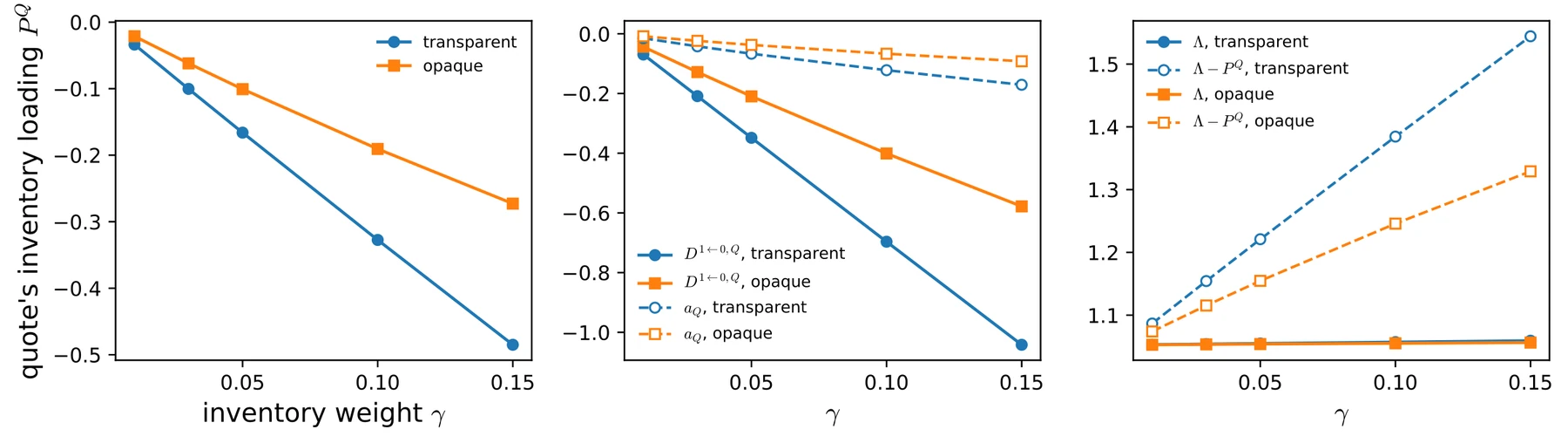
The stationary form of the transparent market is solved on the lag window of Chapter 4, with the trader’s problem exactly as there and the market maker’s quote loading $P^{Q}$ fixed by the origin- $0$ system above in its stationary form. At discount rate $ρ$ the inventory gain is $H^{QQ, 1 \leftarrow 0} = a_{Q} P^{Q} / (a_{Q} - ρ)$ , the market maker’s Riccati equation is algebraic, and the belief row is a linear equation in age with one nonlocal scalar $κ = (H^{W^{0} Q, 1 \leftarrow 0} B^{0⊤}) Σ_{Z}^{- 1/2}$ , the correction to the trader’s inventory loading from how the market maker would filter a departure from it; $P^{Q}$ is then a root of a scalar equation, found by tracking the root in $γ$ upward from the competitive rule. The average-cost limit is degenerate: at $ρ = 0$ the trader’s inventory value equals $P^{Q}$ , its inventory loading responds to $P^{Q}$ with the same slope as the market maker’s rule, and the rule cannot pin $P^{Q}$ . At $ρ = 0.5$ , $ϵ = 0.2$ , unit signal gain and unit noise, a quarter of the impact a trader faces at $γ = 0.1$ is inventory, not information: the market maker’s loading on order flow barely moves, from $1.053$ to $1.057$ , while the net price impact of an order, $Λ - P^{Q}$ , rises from $1.05$ to $1.38$ . Table 6.2 collects the equilibrium at $γ = 0.1$ ; over the range computed the quote loading is linear in the inventory weight, $P^{Q} \approx - 3.3 γ$ for $γ \leq 0.15$ (Figure 6.2). At $γ = 0$ the computation returns the competitive kernels of Chapter 4 to $3 \times 1 0^{- 11}$ , and refining the grid from $60$ to $120$ cells moves $P^{Q}$ by $0.2$ percent. The gain equations admit a second self-consistent gain at $P^{Q} = 0$ , with $a_{Q} \approx - 2.3$ and the trader unwinding inventory it has no reason to touch; the exact best response rules it out, so the competitive rule is the only fixed point of the loop on this branch. Above $γ \approx 0.2$ the trader’s second-order form goes indefinite on this grid at $ϵ = 0.2$ , the same boundary as in Chapter 4, and a larger trading cost is needed to certify larger inventory weights.

The opaque market, computed.

On the lag window the market maker’s problem after its blip, with the trader reading the shading as noise flow, is an ordinary linear-quadratic problem. Its state is the inventory and its own shading history, since the trader’s displaced estimates are a function of the shadings; its control is today’s shading; and the trader’s response to a shading path is its on-path kernel applied to the noise flow it infers by inverting the quote rule, with the signal drift shifted to match. A stationary Riccati equation in $n + 1$ unknowns gives the quote’s inventory loading, and $H^{W^{1} Q, 0}$ and $H^{W^{1} W^{1}, 0}$ are its inventory–history and history–history blocks. With the trader’s privy response in place of the inference, $- 1/ (2 ϵ)$ per unit the quote is raised, the same equation returns the transparent loading to $0.4$ percent at $120$ cells. At $γ = 0.1$ the opaque loading is $P^{Q} = - 0.19$ against $- 0.33$ : the market maker loads its quote on inventory forty percent less when the trader cannot see the flow, and the ratio is $0.6$ over the whole range, $P^{Q} \approx - 1.9 γ$ (Figure 6.2). The reason is the trader’s response to a shading. Read as noise flow, a quote one unit off the rule draws $0.58$ of the order it draws when seen for what it is, and afterwards the trader trades the other way, $+ 0.22$ in total over the window, toward the unwinding it expects and that is not coming. Shading is a weaker tool for managing inventory in the opaque market, so the market maker uses less of it: the trader’s inventory loading is $- 0.40$ against $- 0.70$ , the inventory unwinds at $- 0.076$ against $- 0.12$ , and the net price impact is $1.25$ against $1.38$ . The market maker also loads its optimal quote on its own past shadings, $- 0.04$ on the most recent and decaying, a loading that never fires on the equilibrium path.

Figure 6.2. The stationary transparent and opaque markets against the inventory weight $γ$ ( $ρ = 0.5$ , $ϵ = 0.2$ , unit signal gain and noise, $L = 8$ , $60$ cells). Left: the quote’s inventory loading $P^{Q}$ . Center: the trader’s quote-fixed inventory loading and the inventory’s closed-loop drift. Right: the market maker’s loading on order flow and the net price impact $Λ - P^{Q}$ .

The solvers and figures of this section are the work of Claude Fable 5, a large language model built by Anthropic [7], working under the author’s direction. Interactive versions of the dissertation’s computations are collected at sbabichenko.com/noisestate.

What the pair identifies.

Any difference between the two equilibria is the price of monitoring. Publishing order flow switches the market maker’s wedge off, but it does not discipline the market maker: it loads its quote more on inventory in the transparent market, because a trader who can see the flow can be steered. Most of the gain from being monitored is real inventory efficiency, and the trader’s orders carry the same amount of the fundamental into the price in both markets.

Table 6.3. The two markets at $γ = 0.1$ , at the parameters of Table 6.2. Price profits are gross of a trading cost of $0.13$ in both markets. The information concession is paid through the loading on order flow and the inventory concession through the quote’s inventory loading. The market maker’s loss is flow plus inventory penalty.
	transparent	opaque
trader’s price profits	$1.07$	$1.01$
noise traders’ loss	$1.25$	$1.13$
information concession	$0.96$	$0.95$
inventory concession	$0.30$	$0.17$
market maker’s total loss	$0.28$	$0.63$
$E [Q^{2}] = Σ_{Z} / (2∣ \overset{a}{ˉ}_{Q} ∣)$	$4.7$	$7.5$
expected unwinding rate $\overset{a}{ˉ}_{Q}$	$- 0.106$	$- 0.067$

Table 6.3 gives the accounts at $γ = 0.1$ . The noise traders buy at quotes their own flow has pushed up and sell at quotes it has pushed down. The information concession is the same in the two markets to rounding ( $0.96$ against $0.95$ ), so the inventory concession carries the difference. Transparency transfers about $0.13$ from the noise traders ( $0.30$ against $0.17$ of inventory concession), split evenly between the two strategic players, and separately saves the market maker $0.28$ of real inventory cost, since a trader who can see the flow unwinds the inventory for it.

Which relation holds is an institutional assumption; it does not follow from quotes being actions. A specialist who posts a schedule is monitored; a market maker who prices after seeing the flow is not, and the opaque case is the natural one for the batch auction of Kyle [71]. Existence is known only at the corners; both equilibria above pass the trader’s second-order check of Chapter 4 at each computed $γ$ , the opaque one is the fixed point of the market maker’s Riccati equation, and both rents vanish continuously as $γ \to 0$ . The nearest benchmarks are the monopolist specialist of Glosten [43] for the transparent market, the transparency comparisons of Madhavan [80] and Pagano and Röell [93], and the manipulation of Allen and Gale [3], with the roles reversed, for the opaque one. The comparison is an old policy fight: the London Stock Exchange moved block-trade publication from immediate to next-day and then to a ninety-minute delay between 1987 and 1992, dealers arguing that delayed publication protected the unwinding of their inventory [42].

6.9Conclusion

Allowing some players to monitor a deviation’s origin extends the Chapter 1 deviation calculus to an augmented forward system with two channels. In naive filtering, a naive player misattributes the deviation to primitive shocks and contributes an information wedge. In privy response, a privy player observes the deviation as a labeled zero-variance coordinate and responds through a new kernel. Under perfect transitive monitoring (Assumption 6.4) the seed responses are linear and superposable (Proposition 6.11), and the seed-dependent forward-backward system reduces to a single backward gain sweep that serves all seed times. Section 6.8 works out what monitoring means in a Kyle–Back market.

One direct extension combines this chapter with the delayed public signals of Chapter 2. Suppose an $i$ -origin deviation at time $s$ is initially hidden in an aggregate signal but is identified by a reporting rule at time $s + Δ$ . Before the report, player $j$ is naive to the deviating player, so the seed moves $j$ ’s ordinary noise-state estimate and is priced through the information wedge. At the report, the new information does more than add another measurement row. It attributes an already propagated seed to player $i$ . In the resulting “naive until disclosure, privy afterward” system, origin attribution makes the same delayed transition from hidden influence to disclosure that Chapter 2 derives for signal manipulation.

Two other combinations concern the scale of the calculation. First, translating the rectangular gain into the stationary lag coordinates of Chapter 3 is the bridge to the general strategic-market-maker extension; Section 6.8 does the scalar case. Second, if the dynamics, costs, and transitive monitoring preorder on a finite network are invariant under the graph automorphisms of Chapter 5, the responder–origin gains should inherit an orbit reduction. The stationary rectangular system and the equivariant monitored-response reduction remain open.

The blip convention also makes the chapter a step toward modeling irrationality. A blip is an accidental deviation of variance zero. It is priced, but it occurs with probability zero, so equilibrium behavior never anticipates it. Treating irrationality formally would mean giving blips a variance, which raises the questions of what law the blips follow, whether the naive and privy channels survive when attribution is probabilistic, and how the equilibrium deforms as the blip variance grows from zero.