Chapter 5Local Strategic Information in Symmetric Network Economies

5.1Local strategic information in a large economy

A common large-economy model places many individually negligible agents around a small set of aggregate prices or population statistics. Mean-field methods make this structure tractable by replacing the rest of the population with the distribution of their states [26, 58, 73]. This is natural when interaction is anonymous and the feedback runs through an average state. It is less natural when economic activity is organized into many separate local environments, each containing only a few strategically important players.

A regional credit market may contain only a few major lenders. A local labor market may be dominated by a few employers. A product niche, hospital system, supply-chain cluster, or dealer network may likewise be small as a strategic environment even though each participant is negligible relative to the national economy. Such players are atomistic globally but oligopolistic locally. Their actions can reveal private information to a small set of strategically consequential observers, so each player may alter its action because of what those observers will infer.

The corresponding large-economy limit is large by replication, not by local anonymity. One first solves the finite-player information game inside each local environment and then aggregates its equilibrium outcome across many environments. Aggregating the primitives first can eliminate the local action-to-belief channel that determines behavior inside each market.

This distinction also changes the usual interpretation of local interaction. Centered local shocks may wash out across many markets, but the incentives governing how agents respond to those shocks are repeated. If structurally similar players all attenuate or otherwise distort investment, lending, hiring, or trading because their actions reveal information, the common object is an equilibrium coefficient, not a common private signal. The resulting local distortion can change the conditional cross-sectional mean and the aggregate response to fundamentals as well as the spatial variance.

Figure 1.3 in Chapter 1 shows the equilibrium mean control shifting with signal precision, so information and incentives do not separate. If informational asymmetry is correlated with incentives (sellers of a good being likelier to be experts on it), the correlation shows up in aggregate means.

The symmetry results of Appendix 5.A support this local-to-aggregate architecture. The purchase-order market of Section 5.3 only needs to be solved from the perspective of a representative firm. Chapter 1 removes the hierarchy of forecasts by representing beliefs in noise-state coordinates, the estimated primitive shocks. Graph symmetry reduces the number of unknown kernels: $d_{t} (w, u)$ takes one value per equivalent position of $w$ (Proposition 5.7), while each player still observes only its own channels and moves its neighbors’ posteriors.

The finite-player noise-state equations have several player labels. A policy kernel maps a shock attached to one player into another player’s action response; a filter kernel maps that shock into another player’s estimate; and a belief price prices the effect of changing another player’s posterior. When players occupy the vertices of a homogeneous graph and the model is invariant under graph automorphisms, the relabelings of vertices that preserve the edges, many of these labels describe copies of the same object.

The results of Appendix 5.A concern a finite vertex-transitive graph, one whose symmetries can carry any vertex to any other. They show that the best-response map commutes with graph automorphisms, that a unique equilibrium inherits the graph symmetry, and that policy, filtering, and adjoint kernels take equal values at positions that look alike from the reference player’s seat. Cycles and finite Cayley graphs, graphs whose vertices form a group, admit displacement coordinates. Distance-transitive graphs, whose symmetries can carry any pair of vertices to any equally distant pair, admit distance-shell coordinates.

Dynamic models on financial networks motivate the construction. A close precedent is Feng et al. [36], who solve linear-quadratic stochastic differential games on a directed chain, building on the directed-chain diffusions of Detering et al. [35]. Related network dynamics include interacting diffusions for inter-bank lending [39], systemic-risk mean-field games [27, 28], and contagion with defaults [61]. Here the noise-state, filtering, and information-wedge objects of Chapter 1 inherit the graph’s symmetries. Section 5.3 builds a purchase-order market on the cycle. The strategic effect is signal jamming [40], a shift in mean orders several times the filtering gap.

5.2From local equilibrium to aggregate behavior

5.2.1The spatial mean

On a vertex-transitive graph, a local kernel gives every vertex the same row up to a rearrangement of its entries, so constants map to constants. The spatial mean of $K x$ is therefore the spatial mean of $x$ multiplied by the sum of a single row, $\sum_{r} k (r)$ .

Proposition 5.1 (The spatial mean of a local kernel). Let $Γ$ be a finite group, let $x : Γ \to R^{p}$ , and let $(K x) (v) = r \in Γ \sum k (r) x (v r),$ where $k (r) \in R^{q \times p}$ . Define $\overset{x}{ˉ} = \frac{1}{∣Γ∣} v \in Γ \sum x (v), \overline{K x} = \frac{1}{∣Γ∣} v \in Γ \sum (K x) (v) .$ Then $\overline{K x} = (r \in Γ \sum k (r)) \overset{x}{ˉ} . (5.2.1)$ When $Γ$ is abelian, so that the order of two displacements does not matter, $\sum_{r} k (r)$ is the spatial Fourier transform of the kernel $k$ evaluated at frequency zero.

Proof. For each fixed $r$ , the map $v \mapsto v r$ permutes $Γ$ , so $\frac{1}{∣Γ∣} v \in Γ \sum (K x) (v) = r \in Γ \sum k (r) (\frac{1}{∣Γ∣} v \in Γ \sum x (v r)) = (r \in Γ \sum k (r)) \overset{x}{ˉ} .$ ◻

On a group, after collecting the nonspatial state, source-time, and observer indices, each linear part of the state, filter, policy, and adjoint equations that treats every vertex alike has this form. Proposition 5.1 separates two roles of the equilibrium kernels. Their deviations from the spatial mean govern dispersion, clustering, and propagation across distance. Their spatial mean governs the response of the cross-sectional mean. The first-order condition of Chapter 1 reads schematically as a direct control response plus an information-wedge correction. On a symmetric graph, both pieces generate local kernels in primitive coordinates, the $D_{W}$ of Chapter 1, the form Proposition 5.1 needs. Write $k^{exo}$ for the policy kernel of the exogenous-signal equilibrium (Section 5.4.2); the aggregate loading is $r \sum k^{exo} (r) + r \sum (k (r) - k^{exo} (r)) .$ The kernel shift affects only nonaggregate variation in the special case $r \sum (k (r) - k^{exo} (r)) = 0.$ There is no reason for this cancellation to hold. Players in the same network position share the same incentive to reveal, conceal, exaggerate, or delay, so their distortions point the same way and add up in the mean rather than cancelling. For example, a common productivity component may generate less average investment because each local firm knows that investment reveals information to a few important competitors.

5.2.2Replication across local economies

Consider $M$ local economies indexed by $m$ , each containing the same finite graph $G$ but possibly different local shocks. Let $\overset{ˉ}{D}_{t}^{m, *} = \frac{1}{∣ V ∣} v \in V \sum D_{t}^{m, v, *}$ be the equilibrium average action in local economy $m$ . The macro average is $\overset{ˉ}{D}_{t}^{(M)} = \frac{1}{M} m = 1 \sum M \overset{ˉ}{D}_{t}^{m, *} .$ If, conditional on a common macro history $C_{t}$ , the local economies are identically distributed and conditionally independent with finite second moments, then the conditional law of large numbers gives $\overset{ˉ}{D}_{t}^{(M)} P M \to \infty E [\overset{ˉ}{D}_{t}^{1, *} ∣ C_{t}] . (5.2.2)$ The local noises $W^{0, v}$ average out across local economies, leaving the row sum $\sum_{r} d_{W, t} (r, u)$ of the equilibrium kernels in primitive coordinates, the local form of $D_{W}$ in Chapter 1, applied to the common coordinates.

The order of operations matters. Schematically, $aggregate (local equilibrium) \neq = equilibrium (aggregated local primitives)$ in general.

5.3A purchase-order market on the cycle

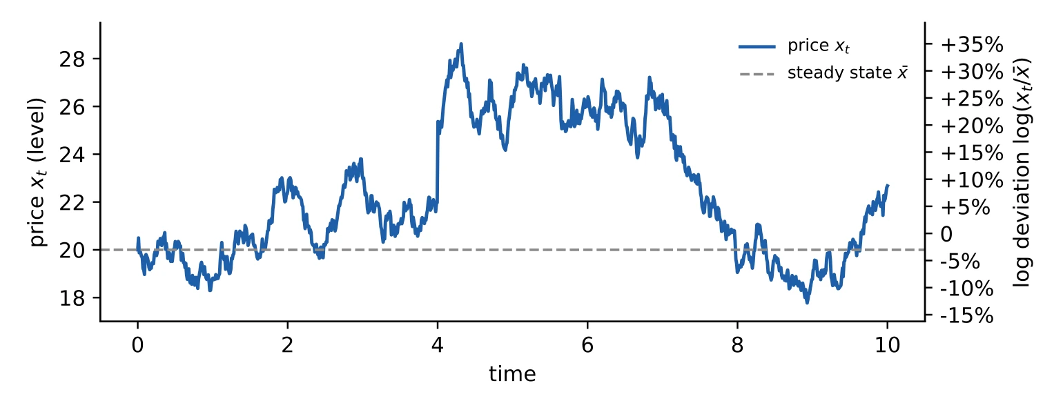
The model of this section is heavily inspired by Woodford [118]. There, firms set prices on the basis of noisy private signals about nominal spending. Because each firm must also forecast what the others will forecast, prices adjust slowly to a monetary shock and the shock has persistent real effects. This section keeps that structure and changes one thing. The signal about nominal spending is no longer an abstract private observation but the market itself, what a firm can see of its own supplier’s quote and its own customer’s order. Those signals are other firms’ actions, the observed actions of Chapter 1, and they travel on the cycle of Appendix 5.B. Firms $v \in Z / N Z$ each buy an input from firm $v - 1$ , sell to firm $v + 1$ and to households, and set prices in advance (Figure 5.2). Every variable is a log deviation from a steady state. If $x_{t}$ is a price or quantity and $\overset{x}{ˉ}$ its value on the constant path the economy would follow without shocks, the variable in the model is $lo g (x_{t} / \overset{x}{ˉ})$ . For small deviations this is the percentage deviation, so a value of $0.01$ means one percent above the steady state. Prices and quantities that multiply in levels add in logs, which makes the relations below linear. Figure 5.1 shows one price in both units. The primitives are quadratic, which keeps the game in the class of Chapter 1.

Figure 5.1. One price in levels (left axis) and as a log deviation from its steady state $\overset{x}{ˉ}$ (right axis), the unit used for every variable in this section.

5.4.1Primitives

Nominal spending $q_{t}$ , the total money households spend per unit time, is a random walk. Firm $v$ has a productivity $a_{t}^{v}$ , the output it gets from a unit of input, and faces a household taste shock $η_{t}^{v}$ , a shift in how much households want its product at a given price. Both are Ornstein–Uhlenbeck, mean-reverting rather than permanent: $d q_{t} = σ_{u} d W_{t}^{q}, d a_{t}^{v} = - θ_{a} a_{t}^{v} d t + σ_{a} d W_{t}^{a, v}, d η_{t}^{v} = - θ_{η} η_{t}^{v} d t + σ_{η} d W_{t}^{η, v}, (5.3.1)$ with $W^{q}$ , $W^{a, v}$ , $W^{η, v}$ independent Brownian motions, so the shocks are independent across firms and of the aggregate. These $1 + 2 N$ Brownian motions and the observation noises of (5.3.6) below are the only sources of randomness. At each date firm $v$ chooses two controls: a quote $P_{t}^{v}$ , the log price at which it will deliver at $t + τ$ , and an order $o_{t}^{v}$ , the log quantity of input it asks firm $v - 1$ to deliver at $t + τ$ . The delivery lag $τ > 0$ turns each control into a delayed row of the state in the sense of (2.1.5): $π_{t}^{v} = P_{t - τ}^{v}, i_{t}^{v} = o_{t - τ}^{v}, d_{t}^{v} = o_{t - τ}^{v + 1}, (5.3.2)$ the price in force, the input arriving, and the deliveries owed to the customer. The price index, which averages the prices in force, and household demand, the quantity households buy from firm $v$ , are algebraic in these, $P_{t} = \frac{1}{N} v \sum π_{t}^{v}, y_{t}^{H, v} = q_{t} - P_{t} - θ (π_{t}^{v} - P_{t}) + η_{t}^{v}, (5.3.3)$ and firm $v$ ’s output at $t$ is $a_{t - τ}^{v} + i_{t}^{v}$ , since productivity is known when the order is placed. Household demand falls by $θ$ times the firm’s price relative to the others’, so $θ$ measures how readily households switch between firms.

Objective

Firm $v$ sets its price in advance and would like it, once in force, to match a target that moves with the price index, with real activity, and with its own input cost. It sells at a markup, so every unit sold to the customer or to households adds to profit; this is the only reason a seller wants its customer to order more. Output at $t$ was fixed by the order placed at $t - τ$ , but deliveries at $t$ are whatever the customer and the households ask for then, so the two can differ. A shortfall has to be bought at short notice while a surplus is dumped. Orders take effort to place. The input is paid at delivery at the price quoted now, which makes an order dearer when the supplier’s quote is high relative to the prices that will prevail at delivery. Firm $v$ minimizes the expected discounted integral of the flow loss, $L_{t}^{v} = missed price target (π_{t}^{v} - π_{t}^{v *})^{2} markup earned on sales - 2 κ (d_{t}^{v} + y_{t}^{H, v}) + output minus deliveries m (a_{t - τ}^{v} + i_{t}^{v} - d_{t}^{v} - y_{t}^{H, v})^{2} + cost of ordering r (o_{t}^{v})^{2} + order times real input price 2 c o_{t}^{v} (P_{t}^{v - 1} - P_{t + τ}), (5.3.4)$ with target price $π_{t}^{v *} = price index P_{t} + demand pressure ξ (q_{t} - P_{t}) + real cost of the input ζ (π_{t}^{v - 1} - P_{t} - a_{t - τ}^{v}) . (5.3.5)$ The target is the price the firm would choose if it knew everything. A firm that sells a differentiated product prices at its cost plus a markup, and in log deviations from the steady state the markup is a constant that drops out, so the target moves with cost. Cost here is the input: the supplier’s price relative to the index, $π_{t}^{v - 1} - P_{t}$ , less the firm’s own productivity $a_{t - τ}^{v}$ , since a more productive firm needs less input per unit of output. The index enters one for one because a firm whose competitors have all raised their prices can raise its own without losing customers. The output gap $q_{t} - P_{t}$ , spending in excess of prices, is demand pressure. When households are buying more than the economy produces at current prices, each firm can charge more, and $ξ$ is how much. This is the pricing rule of Woodford [118], with $ξ < 1$ so that firms move their prices less than one for one with demand, plus the input-cost term. In the loss, the second term is the first-order part of revenue at markup $κ$ , and the third gives the order its curvature. The last is the second-order part of the input bill. The product of order and real cost is bilinear in the firm’s order and its neighbors’ current quotes, which enter the order’s first-order condition as an exogenous linear process. The price in force $π_{t}^{v} = P_{t - τ}^{v}$ is a lagged own control and is carried as a state coordinate. The order’s first-order condition contributes $c E [P_{t}^{v - 1} - P_{t + τ} ∣ F_{t}^{v}]$ . The buyer orders less when it perceives a high real input price and more when it expects the price index to rise over the lag, so its inflation motive is a term of its own. The buyer must decompose the supplier’s quote into inflation and productivity before acting on it. The loss is convex in the quote through the two squares at $t + τ$ and in the order through $r$ and the mismatch term.

Information

Firm $v$ observes exactly its own productivity, its own actions, and its own prices in force. It observes four noisy channels, $d Y_{t}^{v, k} = S_{t}^{v, k} d t + s_{k} d W_{t}^{v, k}, k = 1, \dots, 4, (5.3.6)$ with $S_{t}^{v, 1} = y_{t}^{H, v}, S_{t}^{v, 2} = P_{t}^{v - 1}, S_{t}^{v, 3} = o_{t}^{v + 1}, S_{t}^{v, 4} = o_{t}^{v - 1} :$ its own household sales; the transaction price on its input, whose noise stands for idiosyncratic freight and discount terms; its order book, whose noise is the orders of small buyers; and its supplier’s upstream order, seen through industry data. The $W^{v, k}$ are Brownian motions independent of everything else, and the noise levels $s_{k}$ are fixed. The last three channels are observations of controls, the rows $B_{m}^{Y} D_{t -}^{m}$ of (3.1.2). No firm observes another firm’s action exactly, and no channel’s noise is another firm’s strategy. Latent to firm $v$ are $q$ , $P$ , $η^{v}$ , the neighbors’ productivities, and the neighbors’ quotes and orders. Firm $v$ ’s information $F_{t}^{v}$ is generated by the four channels, $a^{v}$ , and its own past actions, and a stationary strategy is a linear rule on it, $u_{t}^{v} = \overset{u}{ˉ} + k = 1 \sum 4 \int_{0}^{L} g_{k} (l) d Y_{t - l}^{v, k} + \int_{0}^{L} \overset{g}{^} (l) d W_{t - l}^{a, v}, (5.3.7)$ for each of the two controls, with lags cut off at $L$ .

Figure 5.2. The purchase-order market. Left: the cycle seen from firm $v$ . Goods move to the right; quotes (red) travel with the goods and orders (blue) against them; households buy from each firm. Firm $v$ sees its own productivity and actions exactly and the four channels of (5.3.6) through noise. Right: firm $v$ ’s household market at one date. Demand is the line (5.3.3); supply is fixed by the order placed a lag earlier. At the price in force the gap between the two is the mismatch term of the loss (5.3.4).

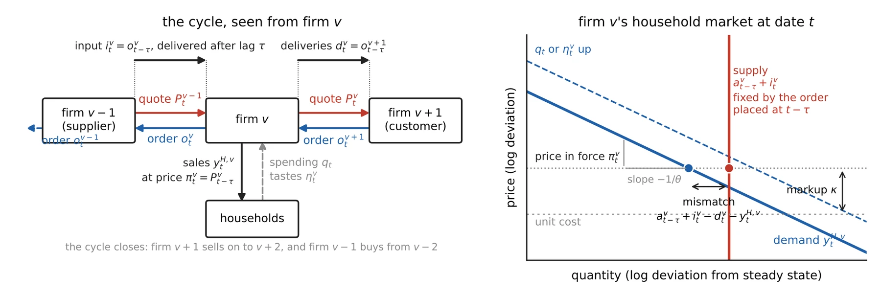
At $t$ the $t - τ$ contracts are delivered; nothing decided at $t$ touches them. The firm reads its channels and its productivity, infers spending and the average of the quotes being made now, and chooses $P_{t}^{v}$ and $o_{t}^{v}$ . Each action carries an information wedge at $t$ and a state price at $t + τ$ , the two terms of the delayed policy line of Chapter 3.

Goods move one way, so the graph is the directed cycle, whose automorphism group is $Z / N Z$ , the rotations, and the displacement reduction of Appendix 5.A applies with signed displacements, with two controls per firm, and with the supplier and the customer in distinct position classes. The kernel of $P$ is the spatial mean of the price-in-force kernels, and $q - P$ is the aggregate object of Proposition 5.1.

Numerical solutions of the purchase-order market

The market of Section 5.3 is solved on a cycle of three firms, inside the rotation-symmetric class of Remark 5.6. The example does for the cycle what the two-player game of Chapter 1 did for the bilateral case.

Primitives

Unless otherwise stated there are $N = 3$ firms, the delivery lag is $τ = 0.5$ , and the objective is the long-run average cost, as in the numerical benchmark of Chapter 3. The shocks (5.3.1) have $σ_{u} = 1$ , $θ_{a} = θ_{η} = 0.5$ and $σ_{a} = σ_{η} = 1$ , so productivity and tastes have stationary standard deviation $1$ and half-life $1.4$ , about three delivery lags. In the loss (5.3.4) and target (5.3.5): $θ = 4$ is the elasticity of household demand to the relative price, $ξ = 0.15$ the weight of the output gap and $ζ = 0.5$ the weight of the real input cost in the target price, $κ = 0.3$ the markup on sales, $m = 1$ the penalty on the gap between output and deliveries, $r = 0.2$ the effort cost of orders, and $c = 0.2$ the coefficient of the input bill. The channel noises in (5.3.6) are $s_{1} = 2.5$ on own sales, $s_{2} = 0.3$ on the transaction price, $s_{3} = 0.3$ on the order book, and $s_{4} = 2$ on the supplier’s upstream order, so a seller sees its customer’s order precisely and a buyer sees its supplier’s order poorly. Strategies take the form (5.3.7) with $L = 24$ . These values are not calibrated. They are chosen so that every channel is active and the equilibrium can be inspected. The signs and orderings below should be trusted and the magnitudes should not.

5.4.2Three information structures

The same shocks and losses are solved under three information structures. Under perfect information every firm observes every primitive shock; there is nothing to filter and no action carries information. Under market information a firm observes only its four channels and its own productivity. The market-information equilibrium is computed twice. In the exogenous-signal version the information wedge is set to zero in every firm’s first-order condition. In this counterfactual, each firm optimizes as though its actions did not change its neighbors’ beliefs. Corollary 1.9 reaches that conclusion when the neighbors’ observations are genuinely unaffected by the firm’s control; here they are not, so the wedge is switched off as a counterfactual rather than vanishing on its own. Firms still filter the same channels; they just cannot teach. In the strategic version the wedge is kept and the neighbors learn from the actions. The strategic shift is the difference between the strategic and the exogenous-signal solutions. The difference between perfect information and the exogenous-signal solution is the filtering gap, the cost of dispersed information without any strategic response to it. Any perfect-information model can be run through the same three steps.

Table 5.1. Mean quote and mean order at $N = 3$ under the three information structures.
	mean quote $\overset{ˉ}{P}$	mean order $\overset{o}{ˉ}$
perfect information	$- 0.260$	$1.298$
market information, exogenous signal	$- 0.252$	$1.261$
market information, strategic	$- 0.274$	$1.036$
strategic shift (strategic $-$ exogenous)	$- 0.022$	$- 0.225$

The cycle length is the one parameter with a direct empirical counterpart. On the cycle each firm is one stage of a production chain that closes on itself, so $N$ is the number of stages. Across $426$ US industries the mean upstreamness, an industry’s average number of stages from final use, $1$ meaning direct sale, is $2.09$ with a standard deviation of $0.85$ and a maximum of $4.65$ [8], so chains of two to five stages cover the bulk of production. Table 5.2 reports the equilibrium over that range and beyond. The order shift is largest at five or six stages, and the quote shift stays between $- 0.012$ and $- 0.022$ . The filtering gap is about $3$ percent at $N = 3$ and $4$ and grows to $6$ percent at $N = 48$ , as more of aggregate spending comes from firms a firm cannot observe. The example uses $N = 3$ , the shortest cycle with a distinct supplier and customer. Nothing below changes qualitatively at other lengths, and the shift at $N = 3$ is the smallest in the range.

Table 5.2. Mean order $\overset{o}{ˉ}$ on cycles of $N$ firms under the three information structures of Section 5.4.2.
$N$
information
signal	strategic
(exo. $-$ perfect)
(strat. $-$ exo.)
3	1.298	1.261	1.036	$- 0.037$	$- 0.225$
4	1.340	1.306	1.018	$- 0.034$	$- 0.289$
5	1.364	1.323	1.020	$- 0.041$	$- 0.303$
6	1.379	1.330	1.027	$- 0.049$	$- 0.303$
8	1.397	1.336	1.043	$- 0.060$	$- 0.293$
12	1.414	1.340	1.062	$- 0.074$	$- 0.278$
24	1.430	1.343	1.079	$- 0.087$	$- 0.264$
48	1.438	1.346	1.090	$- 0.092$	$- 0.256$

5.4.3Mean actions and the strategic shift

Table 5.1 reports the stationary means. Removing perfect information but keeping the exogenous signal lowers the mean order by $3$ percent. Letting the neighbors observe the actions lowers it by a further $18$ percent. As in Chapter 1, movement of the mean action with the information structure is the direct sign that separation fails. Under a separation principle the three rows would coincide. Here the strategic shift is six times the filtering gap.

The order shift comes from the buyer’s side of each link. A firm’s order enters its supplier’s order book, the supplier quotes higher the more demand it infers, and the firm pays more for its input. Each firm therefore orders less than it would if its order were not observed. The mechanism is signal jamming [40, 100]. It is the level distortion of limit pricing [84], in its signaling form, and of career concerns [57]: the distortion fools no one and persists. The noise-state calculus of Chapter 1 adds the magnitude and its comparative statics, which need the filtering dynamics. The quote shift is a tenth the size. The seller’s incentive from Chapter 1, to quote high in the hope that the buyer attributes the quote to inflation rather than to low productivity, is present, but at these parameters the transaction price is a precise signal and a firm already learns most of what it needs to know about the aggregate from its own sales, so the buyer hardly revises its belief when the seller raises its quote.

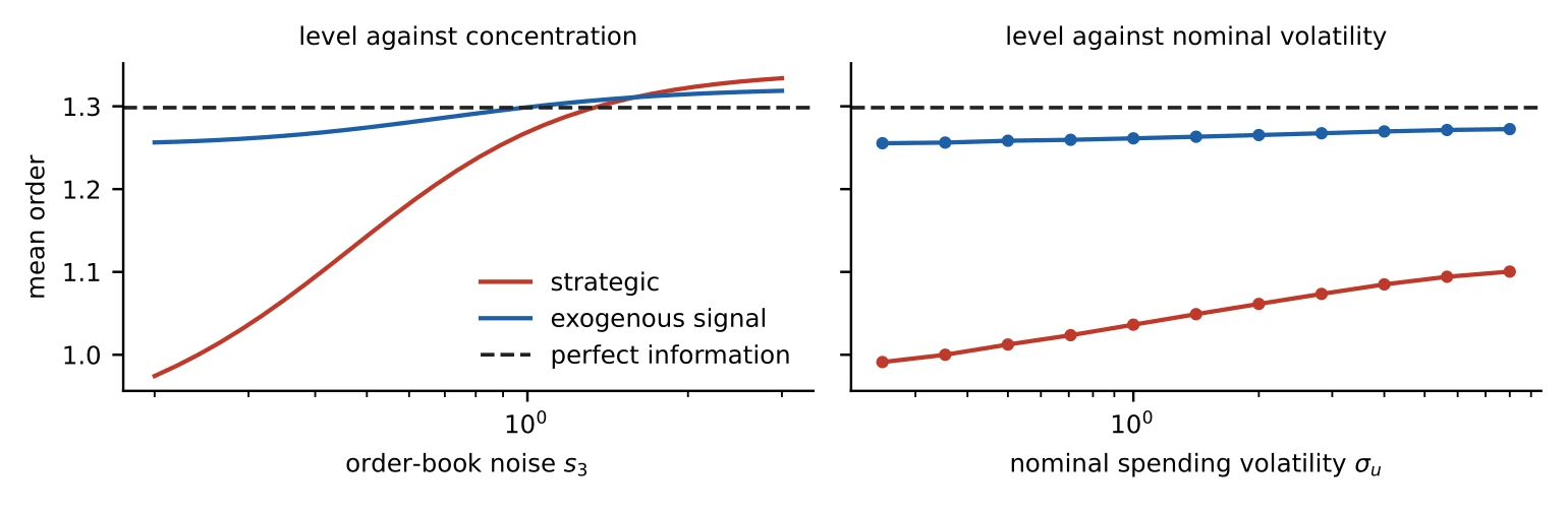
Figure 5.3 plots the mean order against the order-book noise and against the volatility of nominal spending, with the perfect-information level as a reference. With $s_{3} = 0.2$ the order shift is $- 0.28$ ; it crosses zero near $s_{3} = 1.6$ and stays within $0.015$ of zero up to $s_{3} = 3$ . A large $s_{3}$ means the identifiable customer’s order is a small part of the supplier’s order book, the situation of a supplier with many small buyers. In that limit the strategic and exogenous-signal solutions coincide. The model therefore contains the continuum case as a limit. The exogenous-signal level barely moves across either panel, so firms that only filter do not move the mean with these parameters; firms that also manage what their neighbors see do, and their shift shrinks with nominal volatility, from $- 0.264$ at $σ_{u} = 0.25$ to $- 0.172$ at $σ_{u} = 8$ . A supplier reads its order book as a mixture of its customer’s demand and spending, weighting each by its variance. When nominal shocks dominate, a large order is read as inflation and the supplier raises its quote along with the index, which leaves the buyer’s real input price alone, so the buyer has less reason to hold back. The strategic shift depends on the nominal regime in the sense of Lucas [77], Lucas [78]. The delivery lag matters much less. Between $τ = 0.1$ and $τ = 1$ the order shift moves from $- 0.20$ to $- 0.24$ and the quote shift stays at $- 0.022$ . The shift comes from observed actions, not from prices being set in advance.

Figure 5.3. Mean order under the three information structures, against the order-book noise $s_{3}$ (left, log scale) and against the volatility of nominal spending $σ_{u}$ (right, log scale).

5.4.4Impulse responses

The equilibrium kernels are impulse responses to primitive shocks. Figure 5.4 plots the response of the quote index $P_{t + τ}$ to a shock to nominal spending, per unit of the shock, at three levels of nominal volatility and under the three information structures.

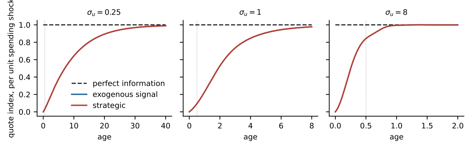
Figure 5.4. Response of the quote index to a unit shock in nominal spending at three volatilities of spending. Dashed: perfect information. Blue: market information with the exogenous signal. Red: strategic. The dotted vertical line marks the delivery lag.

Under perfect information the spending shock raises the quote index by one at once and the price in force by one at lag $τ$ . Household demand is up by one until the prices in force catch up and zero afterwards, so money is neutral apart from the delivery lag. Under market information the index rises slowly, to $0.09$ at $τ$ , $0.53$ at $4 τ$ and $0.98$ at $16 τ$ , and demand decays over the same horizon. The innovation reaches each firm through channels that also carry its idiosyncratic shocks, and firms raise their prices only as fast as they can separate the two. This is the inertia of Woodford [118], produced here by the same higher-order expectations, except that the signals are the neighbors’ quotes and orders. The speed of adjustment is set by the variance of nominal shocks relative to idiosyncratic ones, as in Lucas [77]. At $σ_{u} = 0.25$ the index is at $0.55$ after $16 τ$ and $0.93$ after $46 τ$ ; at $σ_{u} = 8$ it is fully adjusted within two lags. In every panel the strategic kernels lie close to the exogenous-signal kernels. The largest difference is $1.3 \times 1 0^{- 3}$ on a unit shock, and it is not a numerical residual. It is unchanged under a tighter fixed-point tolerance and a finer grid, grows to $2.1 \times 1 0^{- 3}$ at $s_{3} = 0.2$ , and changes sign at $N = 6$ .

The spatial mean of the kernel shift, the object of Proposition 5.1, is present in this economy but small. It is smaller than the response it perturbs by a factor of about $800$ , and smaller than the strategic shift in the mean action, $- 0.225$ , by a factor of about $170$ . The proposition places no bound on its size, and nothing here shows it is small in other economies of the class.

On the spending shock household demand responds by one and output by only $0.045$ . Output is $a_{t - τ}^{v} + i_{t}^{v}$ , fixed by orders placed a lag earlier, so a nominal shock cannot raise it on impact. It raises demand against a fixed supply, and the gap enters the mismatch term of the loss. The real effect of money in this market is a mismatch between deliveries and demand, and it lasts as long as the price adjustment.

On the productivity shock the two market-information solutions do differ (Figure 5.5). Firm $0$ ’s quote falls by $0.38$ on impact, against $0.52$ under perfect information, and the index by a third of that; demand and output rise by about $1.1$ once the lower price is in force. The order rises by $0.18$ on impact and $0.14$ at $τ$ under perfect information, by $0.11$ and $0.06$ under the exogenous signal, and by $0.14$ and $0.08$ in the strategic solution, which also has a second hump at $3 τ$ when the customer’s order returns through the order book. The strategic effect is concentrated in the responses to idiosyncratic innovations, the ones a neighbor cannot distinguish from aggregate conditions except through the firm’s actions, and there the firm responds more, not less. The gap between the strategic and exogenous-signal responses is present at every level of nominal volatility and largest at intermediate levels, where the supplier finds an order hardest to read and the buyer finds it most worth shaping.

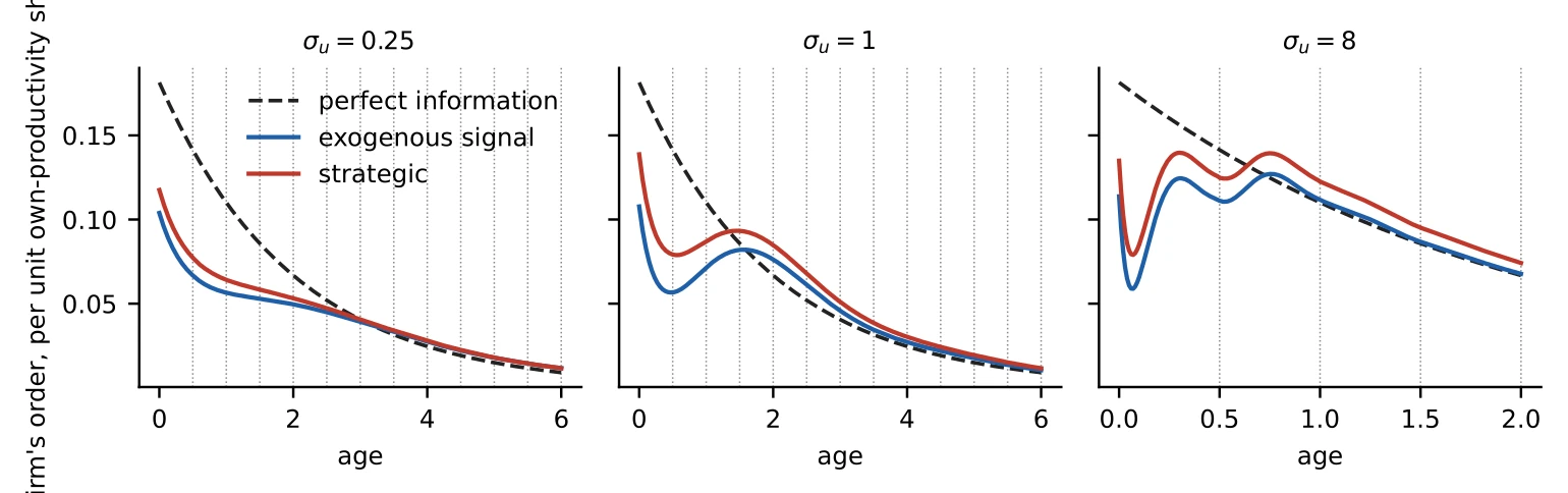
Figure 5.5. Response of firm $0$ ’s order to a unit shock in its own productivity at three volatilities of nominal spending. Dashed: perfect information. Blue: market information with the exogenous signal. Red: strategic. Dotted verticals at multiples of $τ$ .

Table 5.3 collects the size of the kernel shift, the largest difference between the strategic and exogenous-signal kernels, on the two shocks across ten parameter variants. It is largest when the input bill’s cross term $c$ is large or the demand elasticity $θ$ is small, the two places where a nominal level enters the loss other than through a relative price. On the productivity shock it rises with the cost pass-through $ζ$ and with $c$ and falls when own sales are precise. The sales incentive $κ$ leaves every kernel unchanged and moves only the means.

Table 5.3. Largest difference between the strategic and exogenous-signal kernels on the spending shock and on firm $0$ ’s productivity shock, by parameter variant, in units of $1 0^{- 3}$ per unit shock. Each variant changes one parameter from the base case $N = 3$ , $τ = 0.5$ , $θ = 4$ , $ξ = 0.15$ , $ζ = 0.5$ , $κ = 0.3$ , $m = 1$ , $r = 0.2$ , $c = 0.2$ , channel noise $(s_{1}, s_{2}, s_{3}, s_{4}) = (2.5, 0.3, 0.3, 2)$ , $σ_{u} = σ_{a} = σ_{η} = 1$ , $θ_{a} = θ_{η} = 0.5$ .
	spending	own productivity
base	1.3	31
delivery lag $\times 2$ ( $τ = 1$ )	1.5	36
quote on $q$ ( $ξ = 0.5$ )	1.9	16
pass-through $\times 2$ ( $ζ = 1$ )	3.6	55
cross term $\times 3$ ( $c = 0.6$ )	9.7	50
sales incentive $\times 3$ ( $κ = 1$ )	1.3	31
precise sales ( $s_{1} = 1$ )	1.3	3.3
inelastic demand ( $θ = 1$ )	6.7	21
calm spending ( $σ_{u} = 0.25$ )	0.98	14
volatile spending ( $σ_{u} = 8$ )	0.80	21

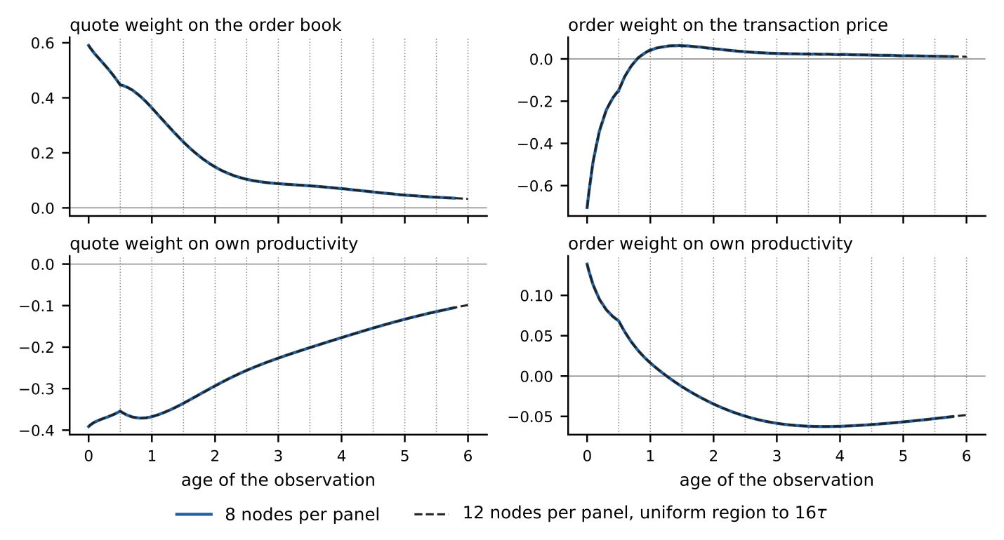
In Figure 5.6 the supplier reads its customer’s order for many lags, which is the channel the order shift runs through, while the buyer reads the transaction price at once and forgets it within one lag. The kinks at multiples of $τ$ in Figure 5.5 and in the policy kernels of Figure 5.6 are produced by the delivery lag. The firm has already acted on an observation older than $τ$ , through the price now in force, and the optimal weight on it changes slope at that age. Each further multiple of $τ$ is one more round of the same effect through the neighbors. The two resolutions in Figure 5.6 are indistinguishable, so the kinks are properties of the equilibrium and not of the discretization.

Figure 5.6. Four policy kernels of the strategic solution, by the age of the observation, at two resolutions of the age grid: the supplier’s quote weight on its order book, the buyer’s order weight on the transaction price, and the quote and order weights on the firm’s own productivity. Dotted verticals at multiples of $τ$ .

5.4.5Computation

The solver is the stationary solver of Chapter 3 extended with the delayed-action and observed-action terms of Section 5.3. Kernels are represented by their values at Chebyshev points on panels in age, with a panel boundary at every multiple of $τ$ up to $8 τ$ and panels of doubling width beyond, out to $L = 24$ . A delay is then an exact shift between panels, and the cost integrals and convolutions are Gauss quadratures on the pieces between breakpoints. The kernels of delayed processes are never resampled onto the grid, which keeps the kinks at multiples of $τ$ exact. The equilibrium is computed as a fixed point of best responses in the control-free parametrization of Chapter 1, in which each best response is a single linear solve, and the fixed point is found by Anderson acceleration. One equilibrium takes about $30$ best responses and two seconds. The cyclic symmetry is used as in Appendix 5.A. The system with every firm on the common strategy is block circulant (each block row is the previous one shifted by one firm), so it is inverted as $N$ independent smaller systems, and the firm whose best response is being computed enters as a low-rank correction.

Recomputing every equilibrium with $12$ nodes per panel and the uniform region extended to $16 τ$ changes the means in the sixth digit and does not move the plotted kernels. Doubling the window to $L = 48$ changes the baseline means in the sixth digit as well. The one exception is the low-volatility case $σ_{u} = 0.25$ , whose price adjustment is slow enough that $L = 24$ truncates it. Its results are computed at $L = 48$ , where they agree with $L = 96$ to three digits. Random starting points converge to the same equilibrium. The leading eigenvalue of the best-response map at the equilibrium has modulus about $0.5$ .

The solvers and figures of this section are the work of Claude Fable 5, a large language model built by Anthropic [7], working under the author’s direction. Interactive versions of the dissertation’s computations are collected at sbabichenko.com/noisestate.

5.5Aggregate interaction and the infinite-network limit

Reducing by graph symmetry keeps who observes whom and how an action changes a particular neighbor’s posterior. Incomplete-information macroeconomics needs this detail, since aggregate dynamics can depend on how dispersed information is converted into actions [5].

Common aggregate effects can enter the vertex equations without changing the spatial indexing. A common factor $C_{t}$ may enter every vertex equation, $d X_{t}^{v} = (\dots + A_{c} C_{t}) d t + σ_{c} d C_{t} + σ d W_{t}^{0, v}, (5.5.1)$ or every observation equation. It acts as common noise for the local graph problem. The relative-position kernels then become conditional on the common history.

Mean-field effects can also sit across local economies. For example, a graph-symmetric state equation may include $A_{m} m_{t}, m_{t} = Law (X_{t}^{o}, D_{t}^{o}, W_{t}^{o} (\cdot, \cdot) ∣ C_{[0, t]}), (5.5.2)$ or a finite-dimensional statistic of that law. The consistency condition comes after the local vertex-transitive reduction: solve the finite strategic-information problem given $(C, m)$ , then require the law of a single local economy to reproduce $m$ .

The finite-cycle formulas suggest an extension from $C_{N}$ to $Z$ , but the finite proof does not itself establish an infinite-player game. Formally one would write $d X_{t}^{v} D_{t}^{v} = (a X_{t}^{v} + β X_{t}^{v - 1} + β X_{t}^{v + 1} + B^{X} D_{t}^{v}) d t + σ d W_{t}^{0, v}, = \overset{ˉ}{D}_{t} + r \in Z \sum \int_{0}^{t} d_{t} (r, u) d W_{t}^{v} (r, u) .$ Turning these displays into a theorem first requires a state space for the spatial process. Spatially homogeneous independent noise is generally not $ℓ^{2} (Z)$ -valued, so the construction needs a weighted space or stationary-random-field formulation even before the strategic fixed point. One must also impose enough decay for the policy and wedge sums to converge and formulate admissible controls and unilateral deviations for infinitely many players. The remaining step is to prove equilibrium existence or convergence of the finite-cycle equilibria. The joint age–displacement representation above suggests one route: obtain estimates uniform in the cycle size for the spatial Fourier transform of the kernels and then invert it.

Conjecture 5.2 (Finite-cycle approximation). Suppose the best-response map is a contraction over short horizons, uniformly in $N$ , that interactions have finite range, and that the filtering, policy, and adjoint kernels decay exponentially in the distance between the two vertices. Then the symmetric equilibria on $C_{N}$ converge locally as $N \to \infty$ to a translation-equivariant equilibrium random field on $Z$ .

5.6Economic implications and conclusion

The local-to-aggregate architecture changes which local quantities count as macroeconomic parameters. Local concentration, observation precision, disclosure delays, and the identity of observable actions can all change the kernel shift. When the same local structure repeats across many markets, these institutional details change aggregate elasticities and means even if technology and preferences are unchanged. In the purchase-order market, the strategic reduction in mean orders is several times the filtering gap, while responses to aggregate shocks barely move.

The adjustment-cost or sluggish-response coefficient that a representative-agent model would fit to the aggregate impulse response is not structural here. It changes when a policy alters local observability or market concentration. This is an information-network version of the usual warning [79] against treating reduced-form aggregate coefficients as policy invariant.

The row sum $\sum_{r} k (r)$ sets the aggregate impulse response and the individual entries $k (r)$ set the covariance between neighbors, so the two together over-identify $k$ . The kernel shift, $k - k^{exo}$ , moves with the information parameters (Table 5.3), which no technological adjustment cost contains.

An intervention need not target a nationally large player to have a macroeconomic effect. A disclosure, privacy, antitrust, or reporting rule can change behavior modestly in every local economy.

The noise-state closes the local hierarchy of beliefs, graph symmetry identifies equivalent positions, and aggregation comes after solving each finite local equilibrium. On a finite vertex-transitive graph, best responses commute with relabeling (Proposition 5.4), a unique equilibrium is invariant under it (Corollary 5.5), and the policy, filtering and adjoint kernels depend on position only relative to the reference player (Proposition 5.7). Local shocks may diversify, but a systematically repeated information incentive can remain in the aggregate response through the kernel’s spatial mean (Proposition 5.1).

5.ASymmetry reduction on a vertex-transitive graph

5.A.1Automorphism-invariant games

Let $G = (V, E)$ be a finite vertex-transitive graph, let $I = V$ be the player set, and fix a reference vertex $o \in V$ . Write $K = Stab (o) = {g \in Aut (G) : g o = o} .$ The stabilizer $K$ collects the relabelings that leave the reference vertex where it is. For $g \in Aut (G)$ , let $U_{g}$ denote the relabeling action on vertex-indexed objects, $(U_{g} x) (v) = x (g^{- 1} v) .$ Relabeling moves each vertex’s object along with the vertex. The same notation applies componentwise to controls, observations, filtrations, strategy profiles, and deterministic kernels.

Assumption 5.3 (Automorphism-invariant game). For every $g \in Aut (G)$ , relabeling all vertex-indexed primitive shocks, initial conditions, state coefficients, observation channels, costs, delays, and admissible strategy sets by $U_{g}$ leaves the game unchanged. If $D$ is admissible, then $U_{g} D$ is admissible, and player $v$ ’s objective under $D$ equals player $gv$ ’s objective under $U_{g} D$ after the same relabeling of primitive randomness.

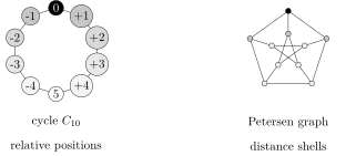
Figure 5.7 illustrates the position classes on two graphs. On a cycle, displacement from the reference vertex labels the vertices, and $\pm r$ share a position class. On a distance-transitive graph such as the Petersen graph, the equivalent positions are the distance shells.

Figure 5.7. Position classes on two graphs. Vertices with the same shade occupy equivalent positions relative to the filled reference player.

5.A.2Relabeling commutes with best response

Equivariant means relabeling before the map matches relabeling after. For a strategy profile $D$ , write $BR (D)$ for the profile whose $v$ th component is player $v$ ’s unique best response to $D^{- v}$ . When individual best responses are not unique, read $BR$ as a correspondence and the equality below as equality of sets.

Proposition 5.4 (Equivariance of the best-response map). Under Assumption 5.3, $BR (U_{g} D) = U_{g} BR (D), g \in Aut (G) . (5.A.1)$

Proof. Fix $g \in Aut (G)$ and a profile $D$ . Let $D^{v}$ be any admissible deviation for player $v$ . Assumption 5.3 gives a bijection between deviations of player $v$ against $D^{- v}$ and deviations of player $gv$ against $(U_{g} D)^{- gv}$ , namely $D^{v} \mapsto U_{g} D^{v}$ . The bijection preserves the objective values. The deviation $D^{v}$ then minimizes player $v$ ’s objective against $D^{- v}$ if and only if $U_{g} D^{v}$ minimizes player $gv$ ’s objective against $(U_{g} D)^{- gv}$ . Applying this statement at every vertex gives (5.A.1). ◻

Corollary 5.5 (Symmetry of a unique equilibrium). Under Assumption 5.3, if the Nash equilibrium $D^{*}$ is unique, then $U_{g} D^{*} = D^{*}, g \in Aut (G) .$

Proof. Because $D^{*} = BR (D^{*})$ , Proposition 5.4 implies $U_{g} D^{*} \in U_{g} BR (D^{*}) = BR (U_{g} D^{*}) .$ The profile $U_{g} D^{*}$ is then also a Nash equilibrium. Uniqueness gives $U_{g} D^{*} = D^{*}$ . ◻

Remark 5.6 (Solving among symmetric profiles). Even without global uniqueness, Proposition 5.4 implies that the subspace of automorphism-invariant profiles is mapped to itself by the best-response map. Any fixed point obtained there is a Nash equilibrium of the original finite game whenever the best-response closure of Chapter 1 applies against arbitrary admissible deviations. Symmetry reduces the deterministic fixed-point problem, but it does not restrict an individual deviating player to symmetric deviations.

Proposition 5.4 says that relabeling the local economy and then solving it gives the same equilibrium as solving first and relabeling afterward. This holds for the endogenous filtering and belief maps as well as for the state dynamics.

5.A.3Kernels indexed by relative position

Fix a graph-symmetric equilibrium. At the reference vertex, write a policy in noise-state coordinates as $D_{t}^{o} = \overset{ˉ}{D}_{t} + w \in V \sum \int_{0}^{t} d_{t} (w, u) d W_{t}^{o} (w, u), W_{t}^{o} (w, u) = E [W_{u}^{w} ∣ F_{t}^{o}] . (5.A.2)$ The kernel $d_{t} (w, u)$ weights the reference player’s estimate of the shock that hit vertex $w$ at time $u$ .

Proposition 5.7 (Stabilizer-orbit reduction). Under Assumption 5.3, let $D^{*}$ be an automorphism-invariant equilibrium, $U_{g} D^{*} = D^{*}$ . Then every deterministic one-point kernel attached to the reference player is constant on $K$ -orbits. Explicitly, $d_{t} (g w, u) = d_{t} (w, u), g \in K . (5.A.3)$ Here $F_{t} (w, w^{'}; u, s)$ is the reference player’s filter kernel from the shock at vertex $w^{'}$ and time $s$ to its estimate of the shock at vertex $w$ and time $u$ , and $H_{t} (w, w^{'}; u)$ is its belief price on player $w$ ’s estimate of the shock at vertex $w^{'}$ and time $u$ . A two-point filter kernel and a two-point belief price are invariant when both vertices are moved by the same automorphism, $F_{t} (g w, g w^{'}; u, s) H_{t} (g w, g w^{'}; u) = F_{t} (w, w^{'}; u, s), = H_{t} (w, w^{'}; u), (5.A.4) (5.A.5)$ for all $g \in K$ .

Proof. Fix $g \in K$ . Since $g o = o$ , the relabeling $U_{g}$ leaves the reference player fixed while permuting every source vertex. The equilibrium is symmetric, $U_{g} D^{*} = D^{*}$ . Apply this identity to the noise-state representation (5.A.2). The blueprint of Chapter 1 is the linear map with deterministic kernel from the primitive shocks $d W$ to the reference player’s estimated shocks $d W^{o}$ ; expanding each estimate through it writes $D^{o}$ on the primitive coordinates, where the deterministic $L^{2}$ representation is unique because the primitive coordinates are orthogonal. The relabeling permutes those coordinates, so the kernel in primitive-shock coordinates agrees at $w$ and $g w$ . The blueprint commutes with $U_{g}$ for $g \in K$ by Assumption 5.3, so composing the primitive-coordinate equality with it gives the same equality for the noise-state kernels on its range, which is (5.A.3). The linear map from source coordinates to the reference player’s conditional estimates defines the filter kernel, so applying the same relabeling simultaneously to its two spatial indices gives (5.A.4). The adjoint equations are the transpose linearization of this equivariant forward system with an invariant quadratic cost source; uniqueness of their solution gives (5.A.5). ◻

Corollary 5.8 (Displacement and distance-shell coordinates). On a finite Cayley graph, group displacement from the reference vertex may index the kernels. On the cycle $C_{N}$ , this gives $D_{t}^{v} = \overset{ˉ}{D}_{t} + r \in Z / N Z \sum \int_{0}^{t} d_{t} (r, u) d W_{t}^{v} (r, u), W_{t}^{v} (r, u) = E [W_{u}^{v + r} ∣ F_{t}^{v}] .$ If the model is also reflection invariant, then $d_{t} (r, u) = d_{t} (- r, u)$ . On a distance-transitive graph, every one-point kernel attached to the reference vertex depends only on graph distance $dist (o, w)$ .

Proof. For a Cayley graph, left translation, multiplying every vertex by a fixed group element, carries any vertex to the reference vertex and converts an ordered pair of vertices into their group displacement. This uses only invariance under the translations; when the model is also reflection invariant, Proposition 5.7 identifies $r$ with $- r$ . In a distance-transitive graph, the symmetries fixing $o$ carry any vertex of a distance shell to any other, so a kernel constant on position classes depends only on $dist (o, w)$ . ◻

The information wedge inherits the same reduction. If $V_{t} (w)$ denotes the contribution of opponent $w$ to the reference player’s wedge, then $V_{t}^{o} = w \neq = o \sum V_{t} (w), V_{t} (g w) = V_{t} (w), g \in K .$ The sum can then be grouped by position class, with each class’s contribution multiplied by the number of positions in it. The number of distinct relative positions controls the number of equilibrium objects, not the number of ordered player pairs.

5.BA finite-cycle market with delayed observation

Take $V = Z / N Z$ . A nearest-neighbor LQG state is $d X_{t}^{v} = (a X_{t}^{v} + β X_{t}^{v - 1} + β X_{t}^{v + 1} + B^{X} D_{t}^{v}) d t + σ d W_{t}^{0, v}, (5.B.1)$ with local observation $d Y_{t}^{v} = B_{X}^{Y} X_{t}^{v} d t + d W_{t}^{v} . (5.B.2)$ All indices are modulo $N$ . Any bounded automorphism-equivariant matrix can replace the nearest-neighbor term: the adjacency matrix, the graph Laplacian, a finite-range convolution. Corollary 5.8 reduces all deterministic one-point kernels to displacement coordinates. Two-point filters and adjoints retain two relative indices because they compare two source locations.

Let each vertex $w$ emit a local signal $d Z_{t}^{w} = C X_{t}^{w} d t + d W_{t}^{Z, w} . (5.B.3)$ Vertex $v$ observes $Z^{w}$ with delay $Δ (v, w)$ . The delay rule is graph symmetric when $Δ (gv, g w) = Δ (v, w), g \in Aut (G) . (5.B.4)$ On the cycle this becomes $Δ (v, w) = Δ_{w - v} .$ At vertex $0$ , the filtration contains $Z_{s}^{r} for s \leq t - Δ_{r} . (5.B.5)$ The filtering equation has birth surfaces $u = t - Δ_{r}, (5.B.6)$ indexed by relative position. Each surface marks the source time at which a delayed signal first enters the filtration. In the finite-player notation these are delayed observation rows. An observation delay small in each local economy can change the equilibrium coefficient at a given relative position and so alter the aggregate response in (5.2.2).

The delayed rows are the local counterpart of Chapter 2, where an observation delay changes the birth and predictable-correction terms of the filter. On a stationary finite cycle, shock age and displacement can jointly index policy, filtering, and adjoint kernels. Spatial Fourier transforms and the temporal transforms of Chapter 3 can then split the linear filtering and adjoint steps into $N$ independent smaller problems. The Kyle–Back market of Chapter 4 is a setting of this kind: a locally informative action also moves an aggregate price.